Goals:
- Introduction to topic modeling, or how to classify texts by shared content (“topics”).
Software
R(install from https://www.r-project.org/)RStudio(install from https://www.rstudio.com/)Java(install from here: https://java.com/en/download/)
Files & Scripts
- The files are on Moodle.
- R script can also be downloaded from here
Class
- Basic explanations
- Hands-on tutorial
Topics
Example 1
Thursday, March 27, 1862
LIGHT ARTILLERY
—I am authorized by the Governor of Virginia to raise a Company of Light Artillery for the war. All those desirous of enlisting in this the most effective arm of the service, would do well to call at once at the office of Johnson & Guigon, Whig Building.
Uniforms and subsistence furnished.
A. B. GUIGON. mh 25—6t
Example 2
Wednesday, August 17, 1864
Royal Marriages.
—There is a story circulated in Germany, and some in Paris, that the match between the heir-apparent of the Imperial throne of Russia and the Princess Dagmar of Denmark having been definitively broken off, another is in the course of negotiation between His Imperial Highness and the Princess Helens of England.
Example 3
Monday, June 22, 1863
NEWS FROM EUROPE.
The steamship Scotia arrived at New York on Thursday from Europe, with foreign news to the 7th inst. The news is not important. The Confederate steamer Lord Clyde was searched by order of the British Government, but nothing contraband being found on board her she was permitted to sail. The Russians have been defeated near Grochoury by the Polish insurgents. The three Powers have sent an earnest note to Russia, asking for a representative Government, a general amnesty, and an immediate cessation of hostilities in Poland.
NB: Before you start running the script!
Run the following lines in R (this will install all necessary packages):
install.packages("rstudioapi")
install.packages("readr")
install.packages("rJava")
install.packages("mallet")
install.packages("plyr")
install.packages("ggplot2")
Topic Modeling Script (Windows Version)
# "Mining the Dispatch," seeks to explore and encourage exploration of the dramatic and often
# traumatic changes as well as the sometimes surprising continuities in the social and political
# life of Civil War Richmond. It uses as its evidence nearly the full run of the Richmond Daily
# Dispatch from the eve of Lincoln's election in November 1860 to the evacuation of the city in
# April 1865. It uses as its principle methodology topic modeling, a computational, probabilistic
# technique to uncover categories and discover patterns in and among texts. On this site you'll
# be able to view and generate graphs and charts that reveal some of the changing patterns in the
# topics that dominated the news during the Civil War in the capital of the Confederacy's
# newspaper of record.

# NB: Required files in a folder:
# dispatch_articles_for_tm_tabular.txt
# dispatch_articles_topic_model_advanced.R
# dispatch_issues_for_tm_stopwords_curated_outOf300.csv

# the following lines
#install.packages("rstudioapi")
library(rstudioapi)
current_path <- getActiveDocumentContext()$path
setwd(dirname(current_path))
print(getwd())

#############################################################################
################# Load Dispatch Articles (one "article" per row) ############
#############################################################################

library(readr)
dispatch.articles <- read.csv(file="dispatch_articles_for_tm_tabular.txt",
                            header=F, sep="\t", quote="",
                            stringsAsFactors=FALSE)

colnames(dispatch.articles) = c("id", "date", "type", "words", "text")

# save as R object
#saveRDS(dispatch.articles,file="dispatch_articles_for_tm_tabular.Rda")
# dispatch.articles <- readRDS(file="dispatch_articles_for_tm_tabular.Rda")

# write.table(dispatch.articles[1:1000,], file = "dispatch_articles_for_tm_tabular_short.txt",
#             row.names=FALSE, na="", quote=FALSE, col.names=TRUE, sep="\t")

#############################################################################
################# MALLET: following http://www.themacroscope.org/?page_id=822
#############################################################################

#install.packages("rJava")
#install.packages("mallet")

#on Windows, mostly
Sys.setenv(JAVA_HOME='C:/Program Files/Java/jre1.8.0_171') # must be the path to Java on your PC
Sys.getenv("JAVA_HOME") # to check the current one
# Some other settings might be in need of correction, like memory
options(java.parameters = "-Xmx8182m")
# loading rJava after!
# rJava or mallet may not load, most likely reasons:
# - 1) need the explicit path to Java (line 50 above);
# - 2) both R and Java must be of the same type either 32 or 64 bit! (for R: check `Tools` > `Global Options`)
library(rJava)
library(mallet)

test = dispatch.articles
#test = dispatch.articles[1:1000,] # comment this one out for full run

test = data.frame(test$id, test$text, stringsAsFactors = F)
colnames(test) = c("id", "text")
mallet.instances <- mallet.import(test$id,
                                  test$text,
                                  "./dispatch_issues_for_tm_stopwords_curated_outOf300.csv", # file with stopwords
                                  FALSE,
                                  token.regexp = "[\\p{L}']+")

# NB: for saving results, especially if you make multiple runs, it makes
#     sense to save file results with appropriate suffixes that would allow
#     to differentiate among different versions of results for post-analysis
#     also, it may make sense to have a spot where you define all your parameters

n.topics <- 40
alphaOptimizationMin <- 20
alphaOptimizationMax <- 50
reiterate <- 100 # change to 100 for test run; 500 (of higher) for better results -- takes much longer
maximization <- 10

# in the file.suffix, you want to save all the parameters that you used for generating
# topic models, namely:
# - n.topics
# - alphaOptimization
# - repetitions / train
#  - maximization parameter (not sure what that one does...)

file.prefix = paste0("tm", n.topics, "_A", alphaOptimizationMin, "_", alphaOptimizationMax,
                     "_iter", reiterate, "_Max", maximization, "_")

# paste0(fileName, file.prefix, extension)

# Starting analysis

topic.model <- MalletLDA(n.topics)
topic.model$loadDocuments(mallet.instances)
vocabulary <- topic.model$getVocabulary()
word.freqs <- mallet.word.freqs(topic.model)
#length(vocabulary)
#vocabulary[1:100]
#head(word.freqs)

#############################################################################
# stopwords: run if no stopword list is available ###########################
# stopwords = as.data.frame(word.freqs)
# stopwords = stopwords[with(stopwords, order(-term.freq)), ]
# stopwords = data.frame(stopwords$words)
# write.table(stopwords, file = "dispatch_issues_for_topic_model_stopwords_new.csv", row.names=FALSE, na="", quote=FALSE, col.names=TRUE, sep="\t")
# this is a full list/table, which needs to be trimmed manually #############
#############################################################################

#############################################################################
# The following three lines of code will take a while to run ################
### the higher VAL in topic.model$train(VAL), the longer it takes ###########
### the optimal seems to be 500; leave it overnight :) ######################
#############################################################################

topic.model$setAlphaOptimization(alphaOptimizationMin, alphaOptimizationMax)
topic.model$train(reiterate) #initial: 200; the higher the number the longer it takes to finish
# with 200 iterations, and all issues (~1300), Total time is: 5 minutes 15 seconds
# with 500 iterations, and all articles (~140k): Total time: 11-12 minutes
# (on MacBook Pro, i7, 16Gb RAM)
topic.model$maximize(maximization)

# Continue analysis

doc.topics <- mallet.doc.topics(topic.model, smoothed=T, normalized=T)
topic.words <- mallet.topic.words(topic.model, smoothed=T, normalized=T)

topic.docs <- t(doc.topics)
topic.docs <- topic.docs / rowSums(topic.docs)
write.csv(topic.docs, paste0("./", file.prefix, "topics-docs-articles.csv"))

# Get a vector containing short names for the topics
topics.labels <- rep("", n.topics)
topics.label.length <- 5
for (topic in 1:n.topics) topics.labels[topic] <- paste(mallet.top.words(topic.model, topic.words[topic,], num.top.words=topics.label.length)$words, collapse=", ")
## cluster based on shared words
plot(hclust(dist(topic.words)), labels=topics.labels)

#############################################################################
# this will save an image of the dendrogram #################################
png("dendrogram_of_topics.png", width=1500, height=1500, res=200)
plot(hclust(dist(topic.words)), labels=topics.labels)
dev.off()
#############################################################################

# Get a vector containing longer names for the topics
topics.labels <- rep("", n.topics)
topics.label.length <- 15
for (topic in 1:n.topics) topics.labels[topic] <- paste(mallet.top.words(topic.model, topic.words[topic,], num.top.words=topics.label.length)$words, collapse=", ")

# have a look at keywords for each topic
topics.labels

# write these to a file
write.csv(topics.labels, paste0("./", file.prefix, "topics-labels-articles.csv"))
topics.labels <- read.csv(file=paste0("./", file.prefix, "topics-labels-articles.csv"),
                          header=TRUE, sep=",", quote='"', stringsAsFactors=FALSE)

# create data.frame with columns as documents and rows as topics
topic_docs <- data.frame(topic.docs)
names(topic_docs) <- test$id

# Further analysis
topics.docs.dates = as.data.frame(t(topic_docs))

# converting from factor to numeric
indx <- sapply(topics.docs.dates, is.factor)
topics.docs.dates[indx] <- lapply(topics.docs.dates[indx], function(x) as.numeric(as.character(x)))

topics.docs.dates = cbind(rownames(topics.docs.dates), topics.docs.dates)
# ids are in topics.docs.dates[,1]
# topics are in topics.docs.dates$V+number
rownames(topics.docs.dates) <- NULL


# JOIN TM TABLE WITH INITIAL DATA!
topics.texts.stats = topics.docs.dates
names(topics.texts.stats)[1] = "id"
# fixing some ID corruption (1864-02-10_article_96 becomes X1864.02.10_article_96)
topics.texts.stats$id = as.character(topics.texts.stats$id)
topics.texts.stats$id = sub("^X", "", topics.texts.stats$id)
topics.texts.stats$id = sub("\\.", "-", topics.texts.stats$id)
topics.texts.stats$id = sub("\\.", "-", topics.texts.stats$id)
topics.texts.stats.complete = merge(topics.texts.stats, dispatch.articles, by="id")

# reading top samples of topics
# - rearrange the table for V40
topics.texts.stats.complete = topics.texts.stats.complete[order(-topics.texts.stats.complete$V40),]
# - print out top 5 samples for V40
topics.texts.stats.complete$text[1:5]

# saving
write.table(topics.texts.stats.complete, file = paste0("./", file.prefix, "topics_docs_dates.txt"),
            row.names=FALSE, na="", quote=FALSE, col.names=TRUE, sep="\t")

# if you have already run the TM process, you can load the results with the following line:
topics.texts.stats.complete <- read.csv(file=paste0("./", file.prefix, "topics_docs_dates.txt"),
                            header=TRUE, sep="\t", quote="",
                            stringsAsFactors=FALSE)
# save as R object
#saveRDS(topics.texts.stats.complete,file=paste0("./", file.prefix, "topics.texts.stats.complete.Rda"))
# read back R object
#topics.texts.stats.complete <- readRDS(file=paste0("./", file.prefix, "topics.texts.stats.complete.Rda"))

####################################################################################################
# Plotting topics over time ########################################################################
# Visualization cookbook: http://r-statistics.co/Top50-Ggplot2-Visualizations-MasterList-R-Code.html
####################################################################################################

library(plyr)
library(ggplot2)

# to graph topics over time the main table must be modified:
# - topic values must be summed up for each day
# -- remove unnecessary columns
topics.texts.stats.cumulative = subset(topics.texts.stats.complete, select = -c(id, type, words, text))
# - focus on the period of the Civil War
topics.texts.stats.cumulative$date = as.Date(topics.texts.stats.cumulative$date)
# American Civil War: Apr 12, 1861 - May 13, 1865
topics.texts.stats.cumulative = topics.texts.stats.cumulative[
  which(topics.texts.stats.cumulative$date >= as.Date("1860-11-01") &
          topics.texts.stats.cumulative$date <= as.Date("1865-04-30")), ]
# calculating total sum of topics per each article
topics.texts.stats.cumulative$total = rowSums(topics.texts.stats.cumulative[1:n.topics])

# Try numbers from 1 to 40 (or higher, if you changed the number of topics)

topic.var = 9
plotting.data = topics.texts.stats.cumulative
plotting.data.var = count(plotting.data, vars=c("date"), wt_var = sprintf("V%d", topic.var))
names(plotting.data.var) = c("date", "var")
plotting.data.tot = count(plotting.data, vars=c("date"), wt_var = "total")
names(plotting.data.tot) = c("date", "tot")
plotting.data.fin = merge(plotting.data.var, plotting.data.tot, by="date")

ggplot(plotting.data.fin, aes(x=date, y=var/tot*100)) +
  geom_line(aes(y=var/tot*100), col="gray") +
  geom_smooth(method="loess", span = 0.1, col="blue") +
  labs(title=paste0("Topic ",topic.var," Over Time"),
       subtitle=paste("Topic Words:", topics.labels[topic.var,][2]),
       caption="Source: Richmond Dispatch (Americal Civil War Period)",
       y="Frequencies %")

# save the graph
graph.name = paste0(file.prefix, "Topic_", topic.var, ".png")
ggsave(graph.name, width = 10, height = 5, dpi = 300)

# Now print out a few top samples of a topic
topics.texts.stats.complete = topics.texts.stats.complete[order(-topics.texts.stats.complete[,topic.var+1]),]
topics.texts.stats.complete$text[1:5]

### GENERATE ALL GRAPHS IN A LOOP ###

for(i in seq(1, 40, 1)){
  topic.var = i
  plotting.data = topics.texts.stats.cumulative
  plotting.data.var = count(plotting.data, vars=c("date"), wt_var = sprintf("V%d", topic.var))
  names(plotting.data.var) = c("date", "var")
  plotting.data.tot = count(plotting.data, vars=c("date"), wt_var = "total")
  names(plotting.data.tot) = c("date", "tot")
  plotting.data.fin = merge(plotting.data.var, plotting.data.tot, by="date")

  ggplot(plotting.data.fin, aes(x=date, y=var/tot*100)) +
    geom_line(aes(y=var/tot*100), col="gray") +
    geom_smooth(method="loess", span = 0.1, col="blue") +
    labs(title=paste0("Topic ",topic.var," Over Time"),
         subtitle=paste("Topic Words:", topics.labels[topic.var,][2]),
         caption="Source: Richmond Dispatch (Americal Civil War Period)",
         y="Frequencies %")

  # save the graph
  graph.name = paste0(file.prefix, "Topic_", topic.var, ".png")
  ggsave(graph.name, width = 10, height = 5, dpi = 300)
}
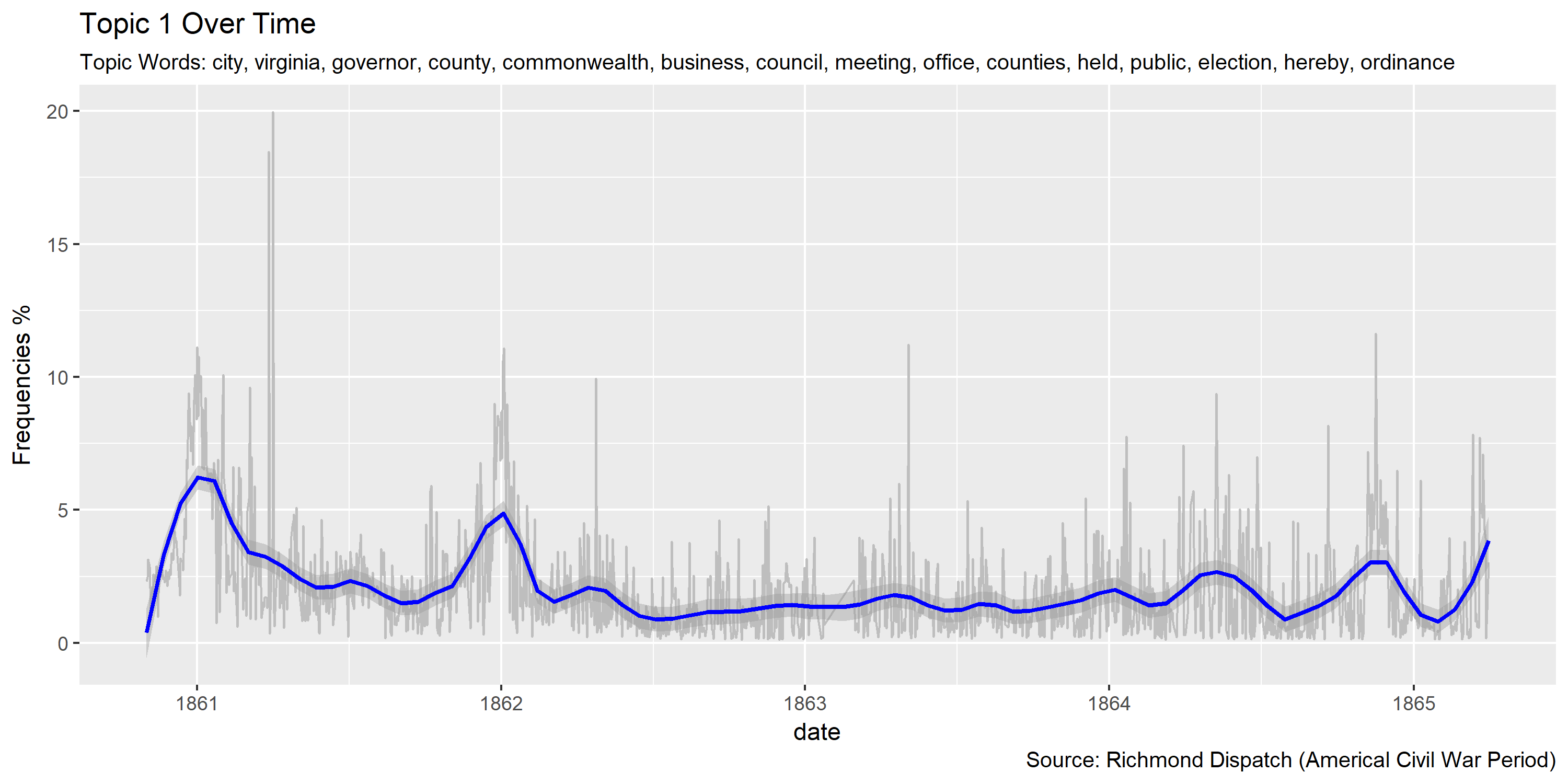
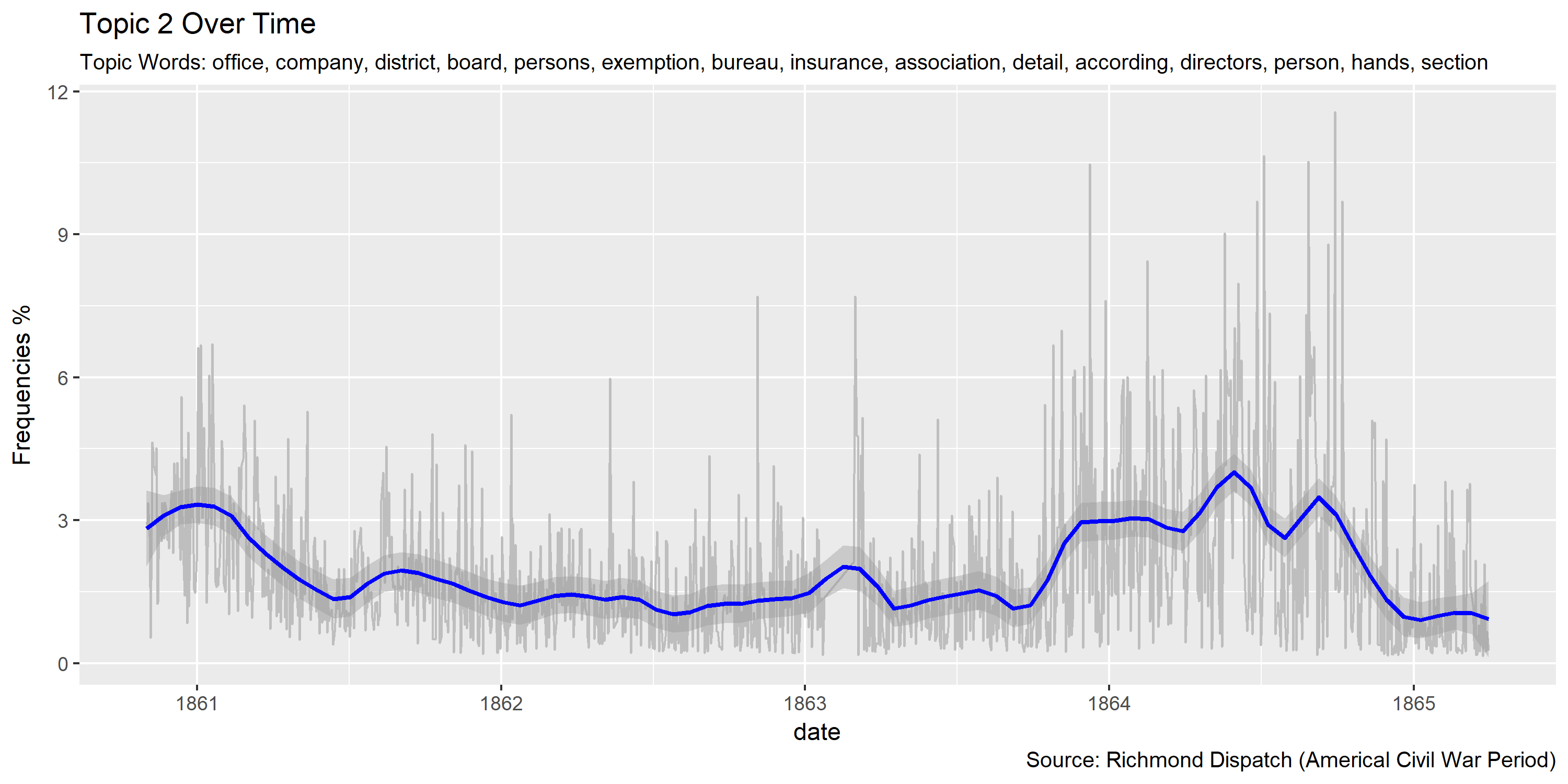
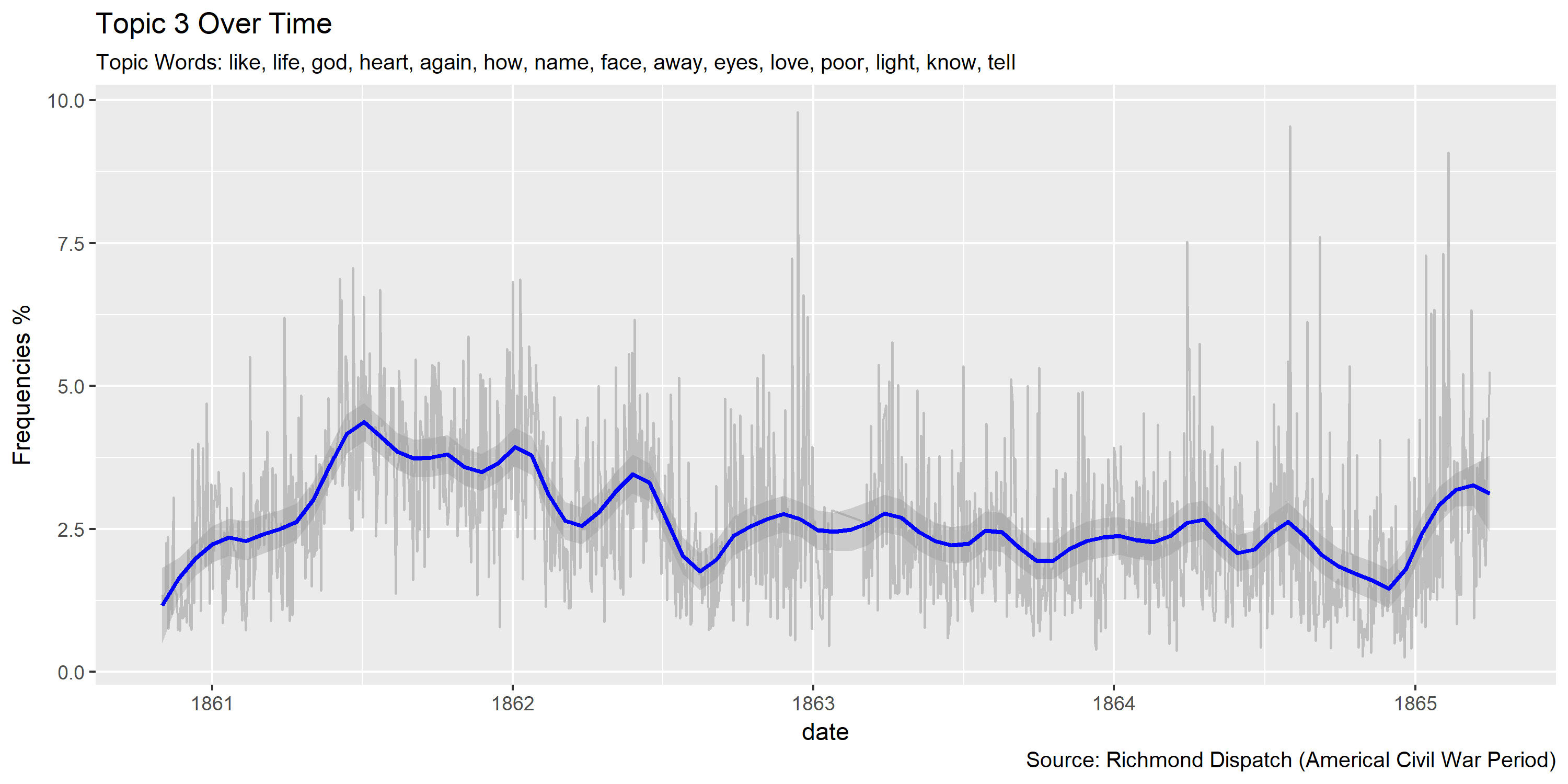
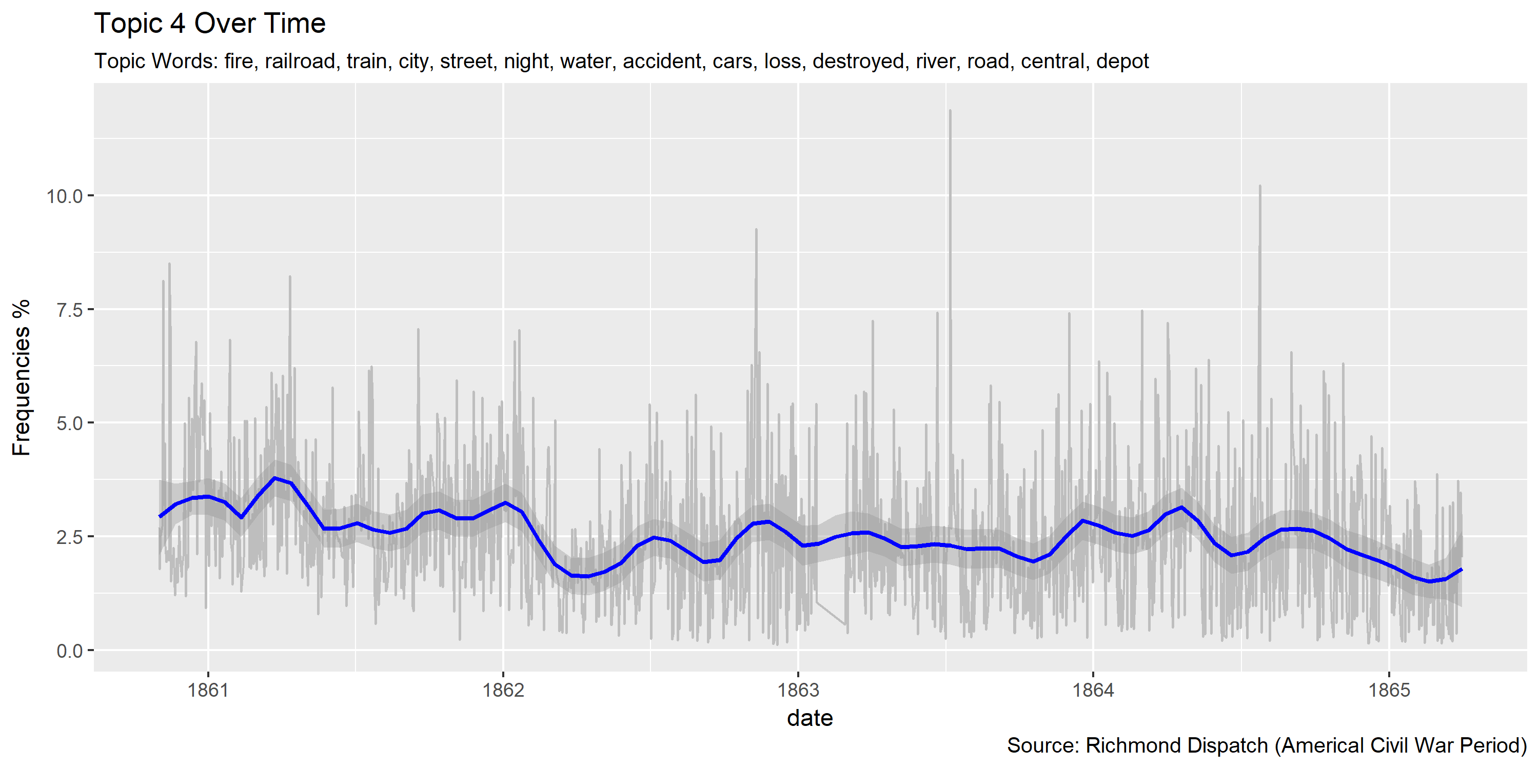
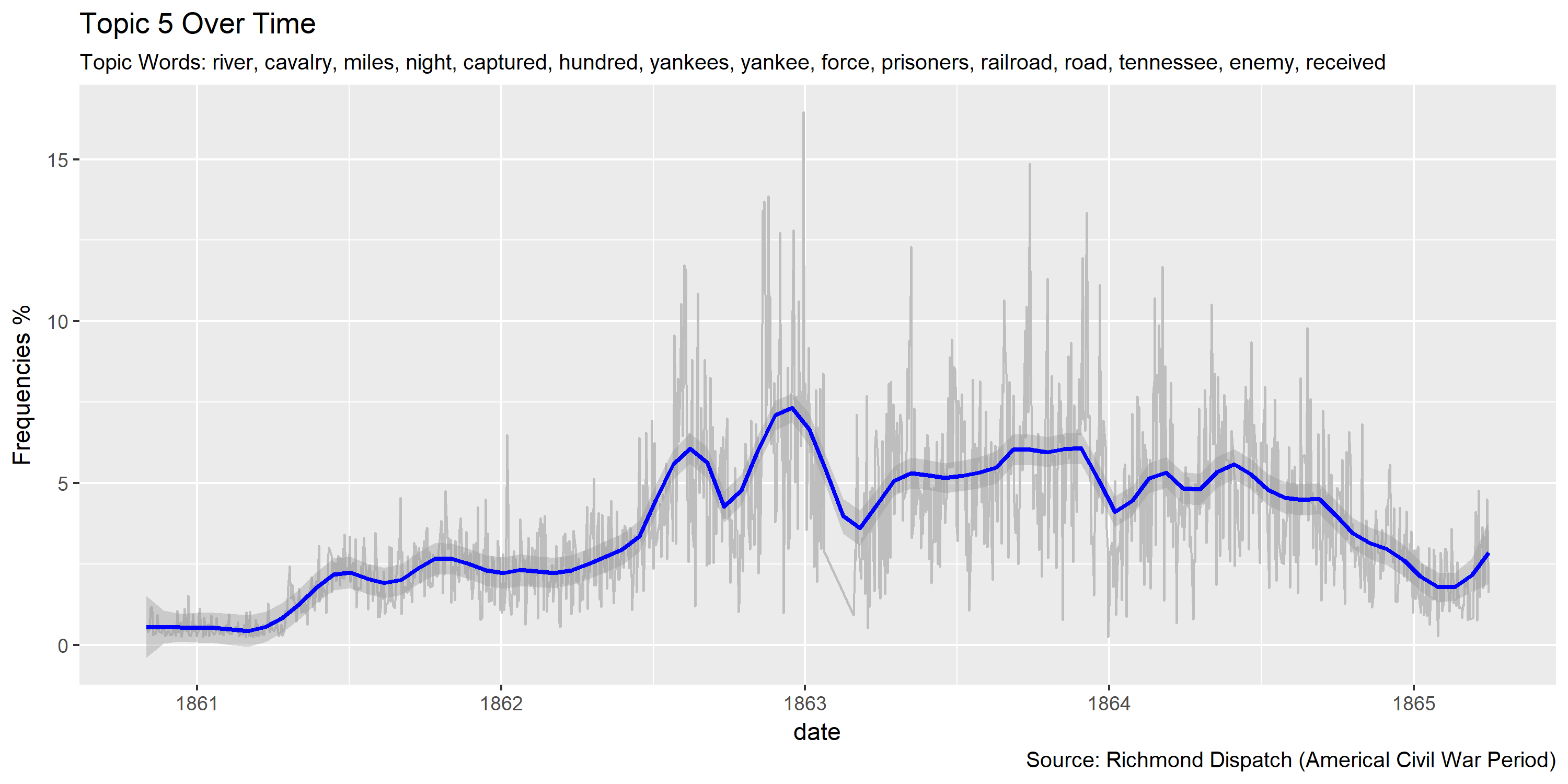
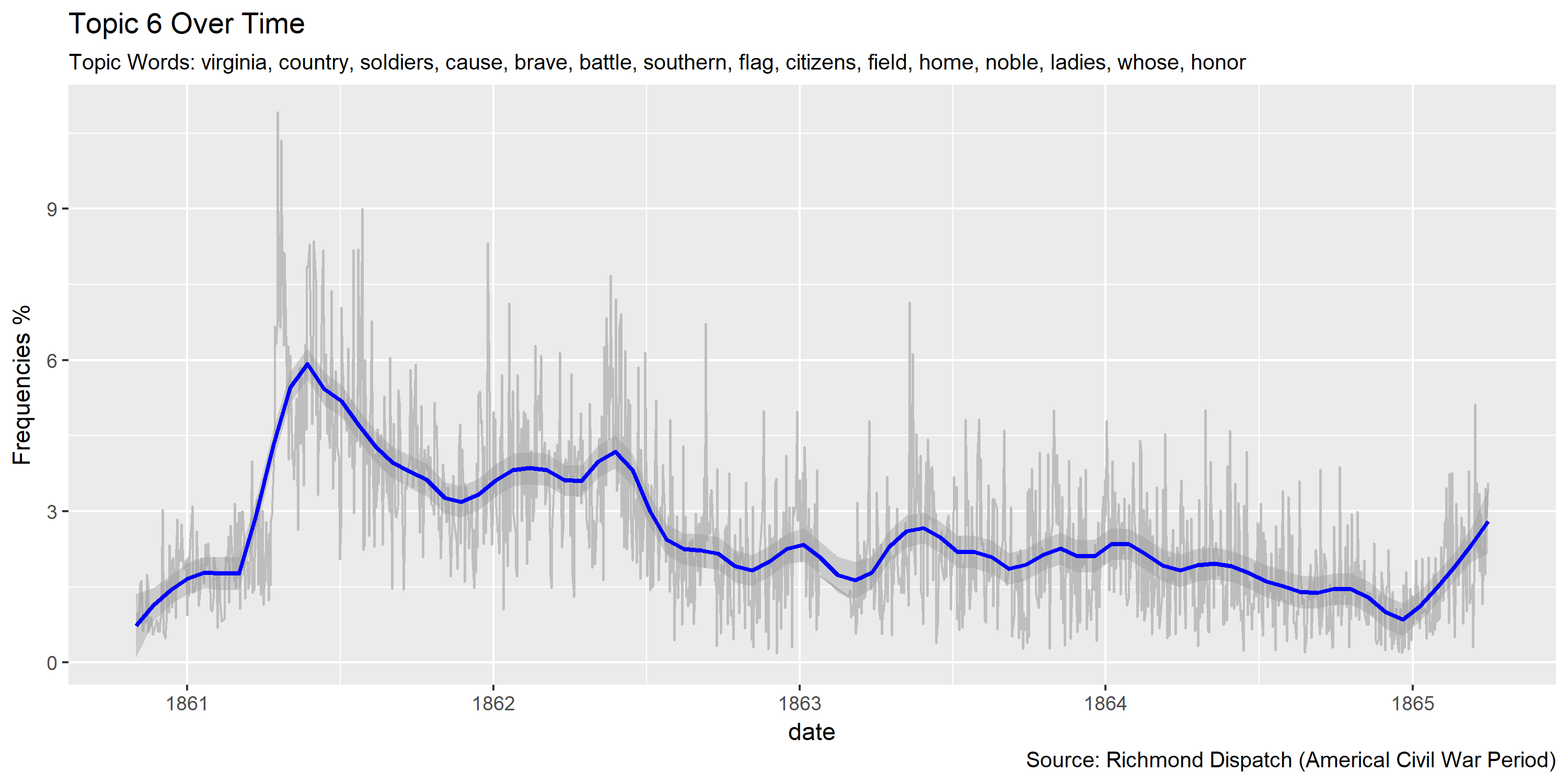
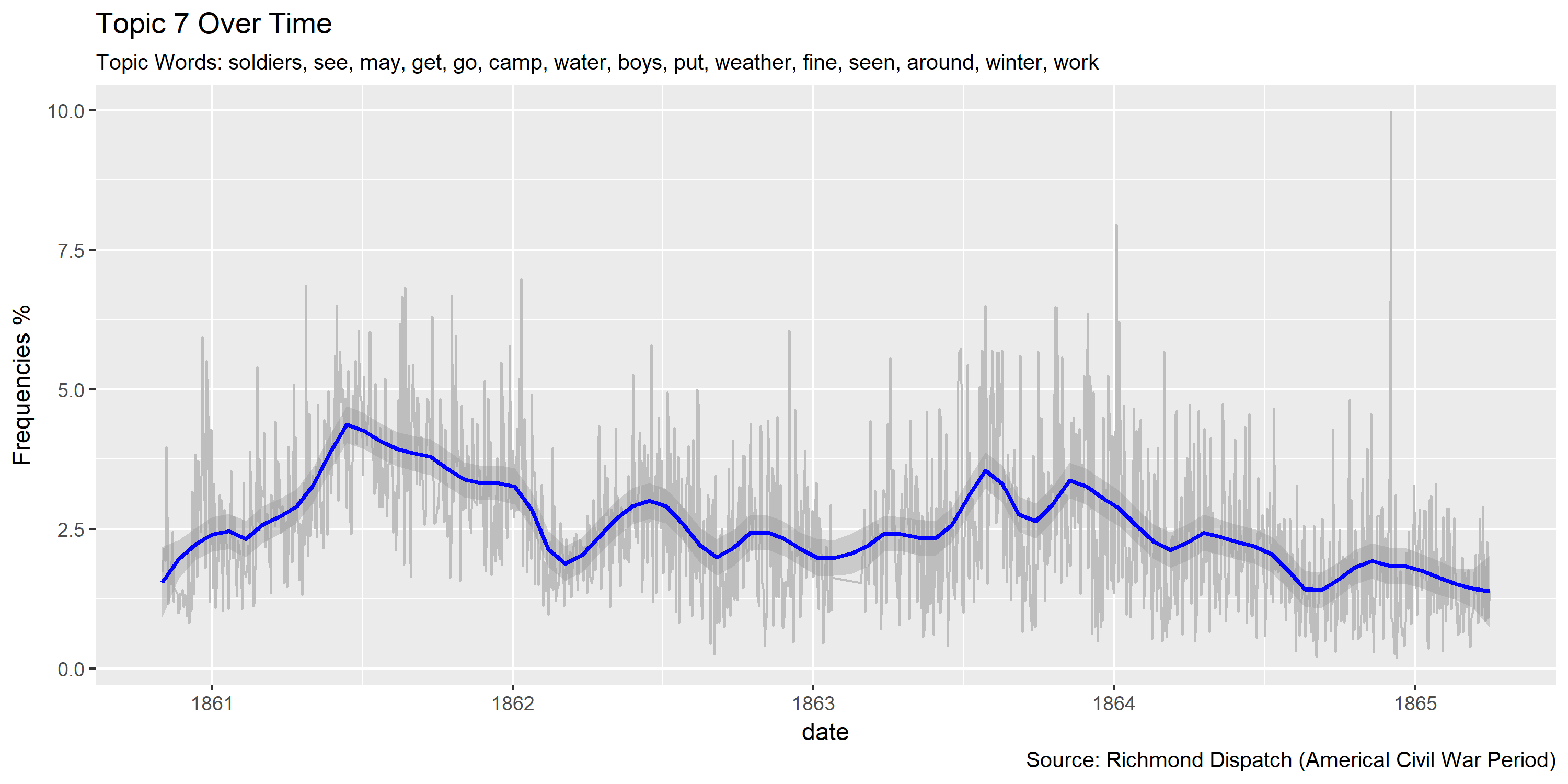
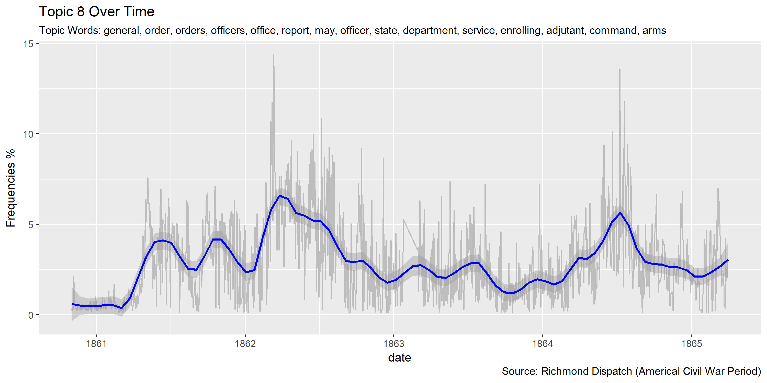
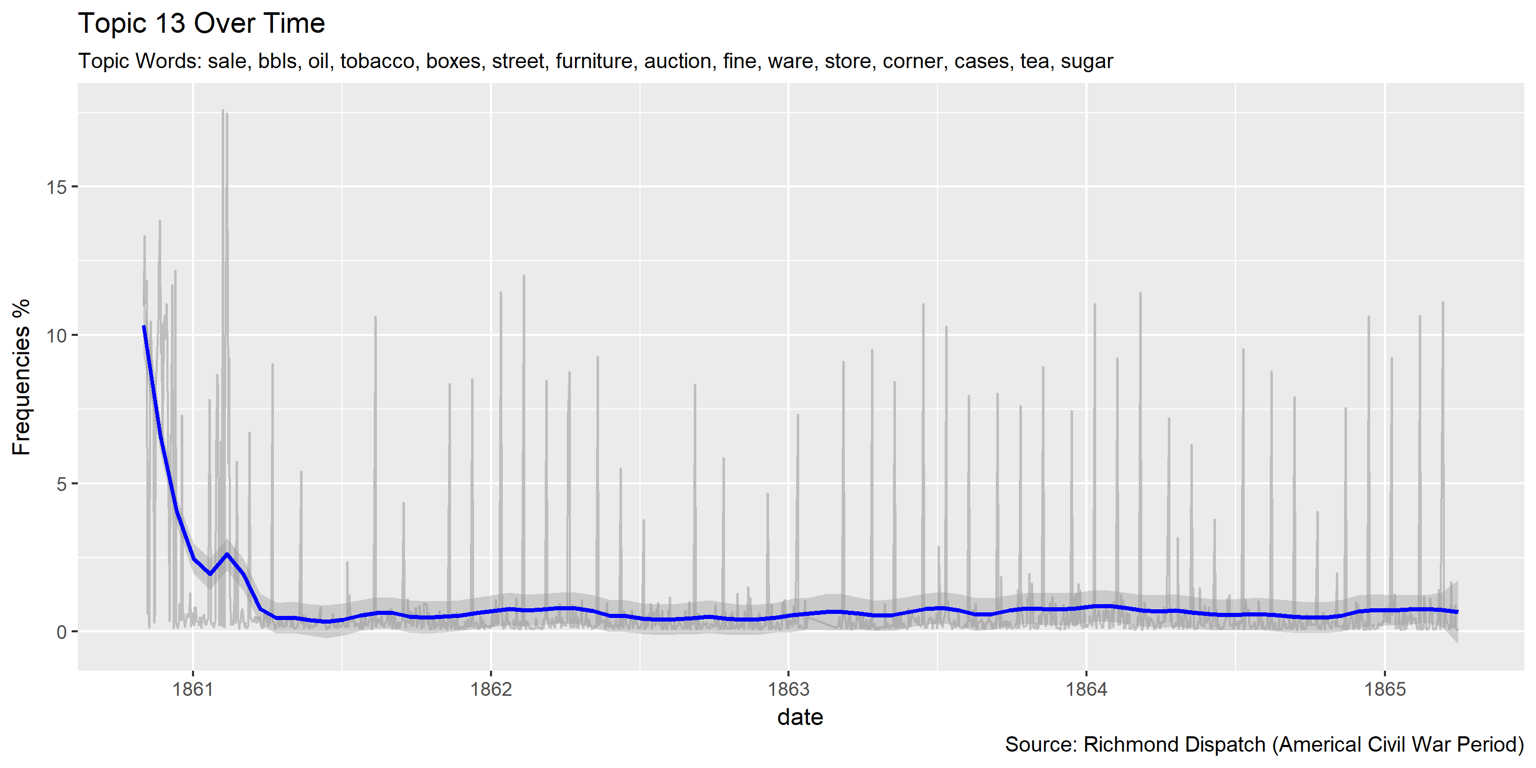
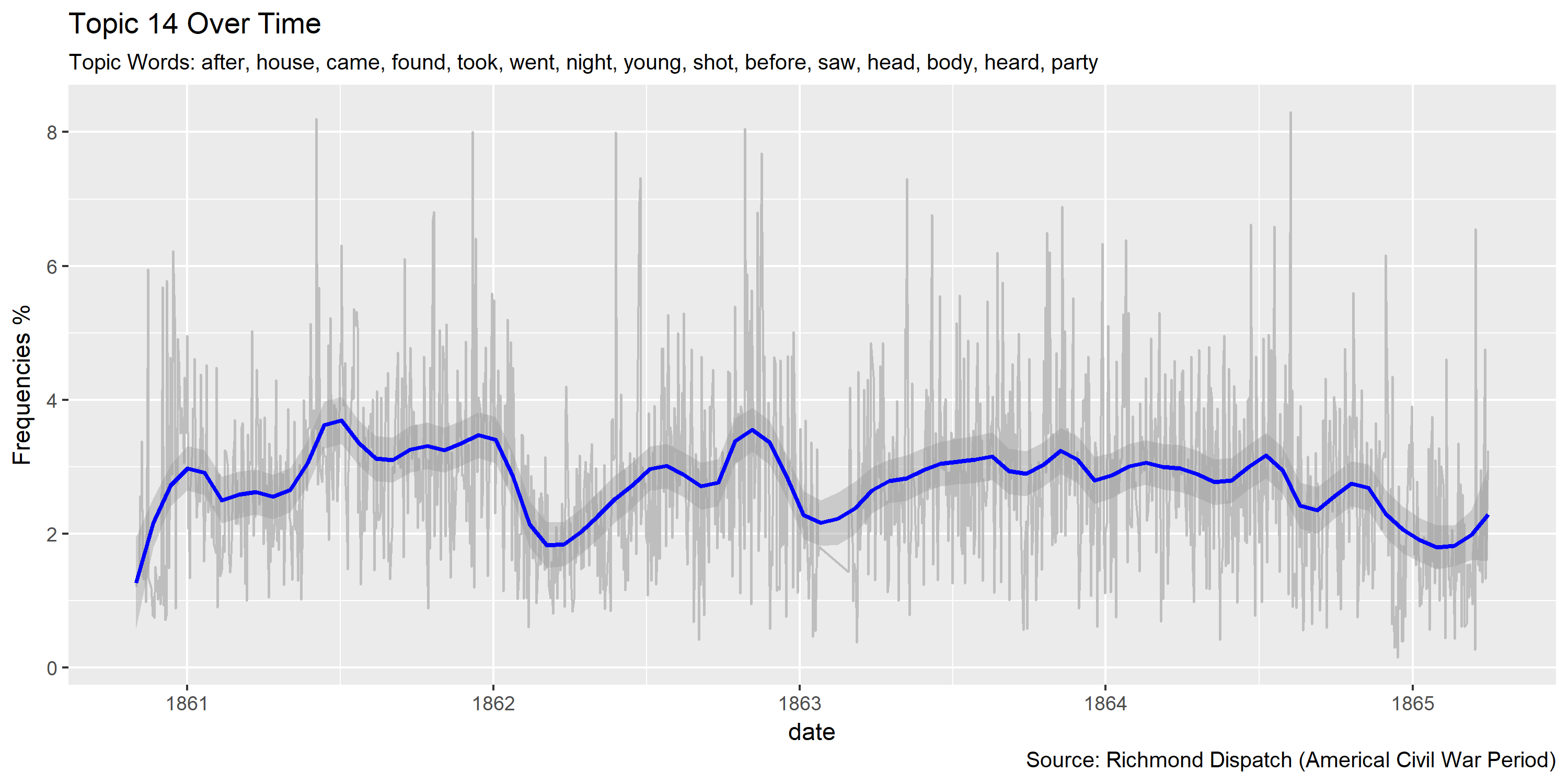
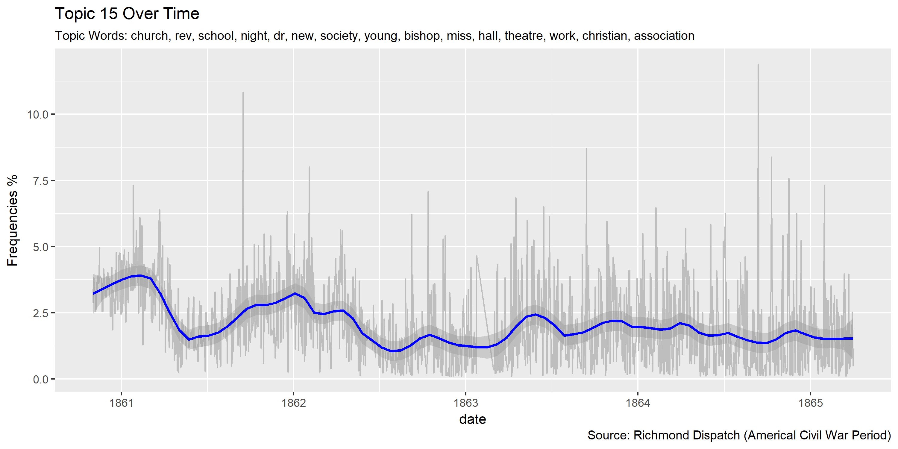
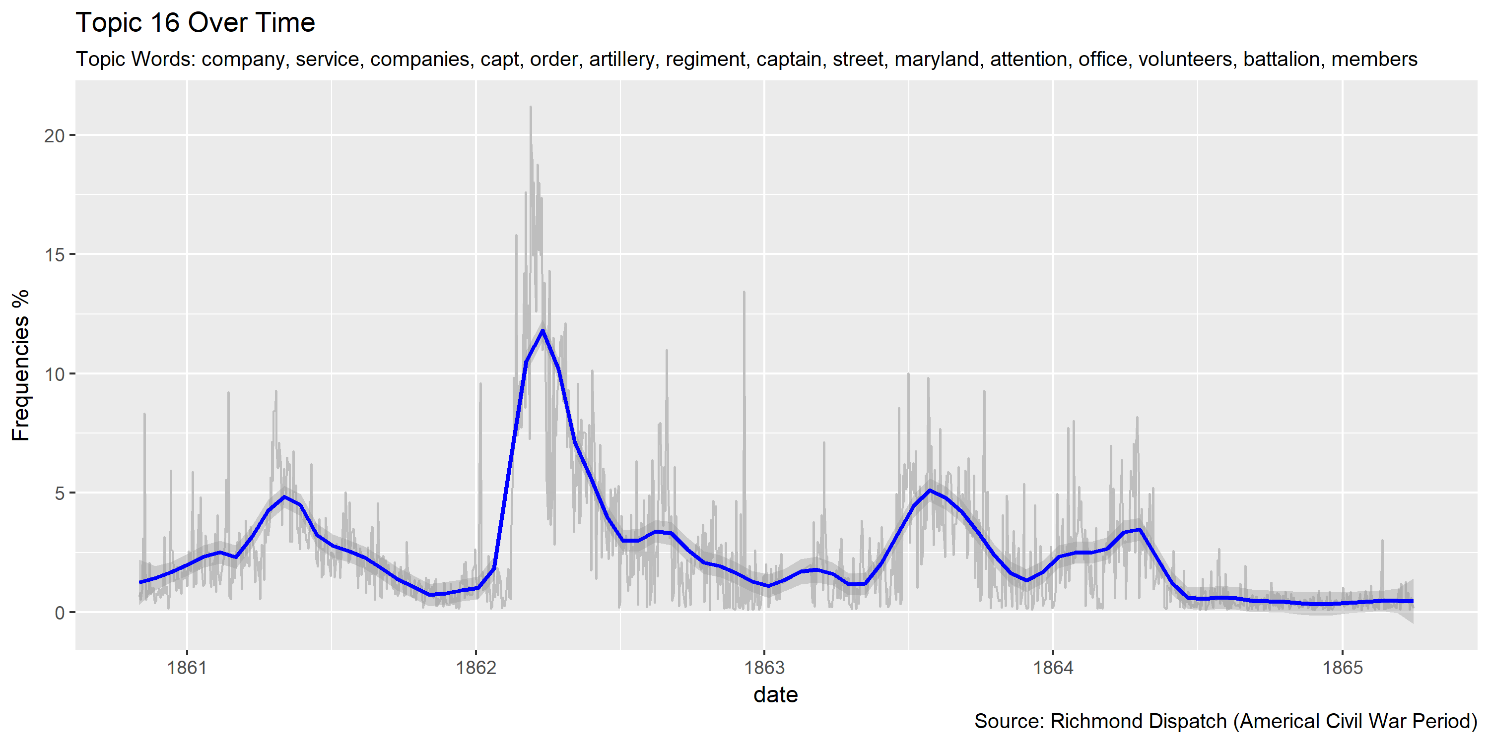
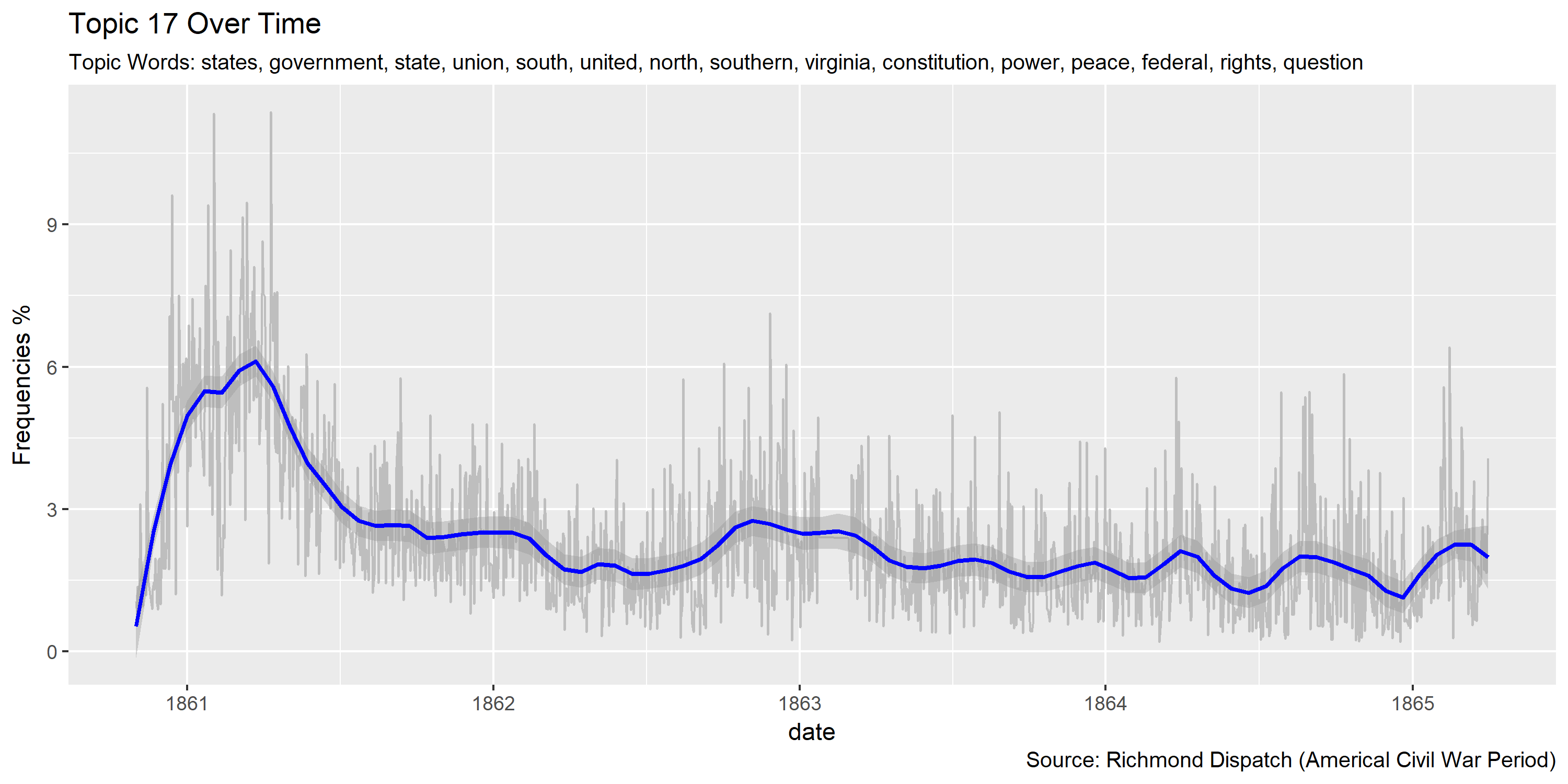
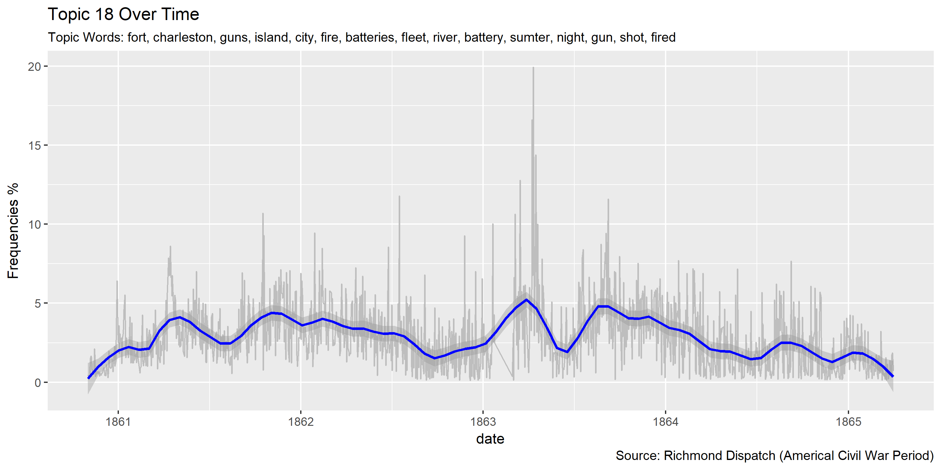
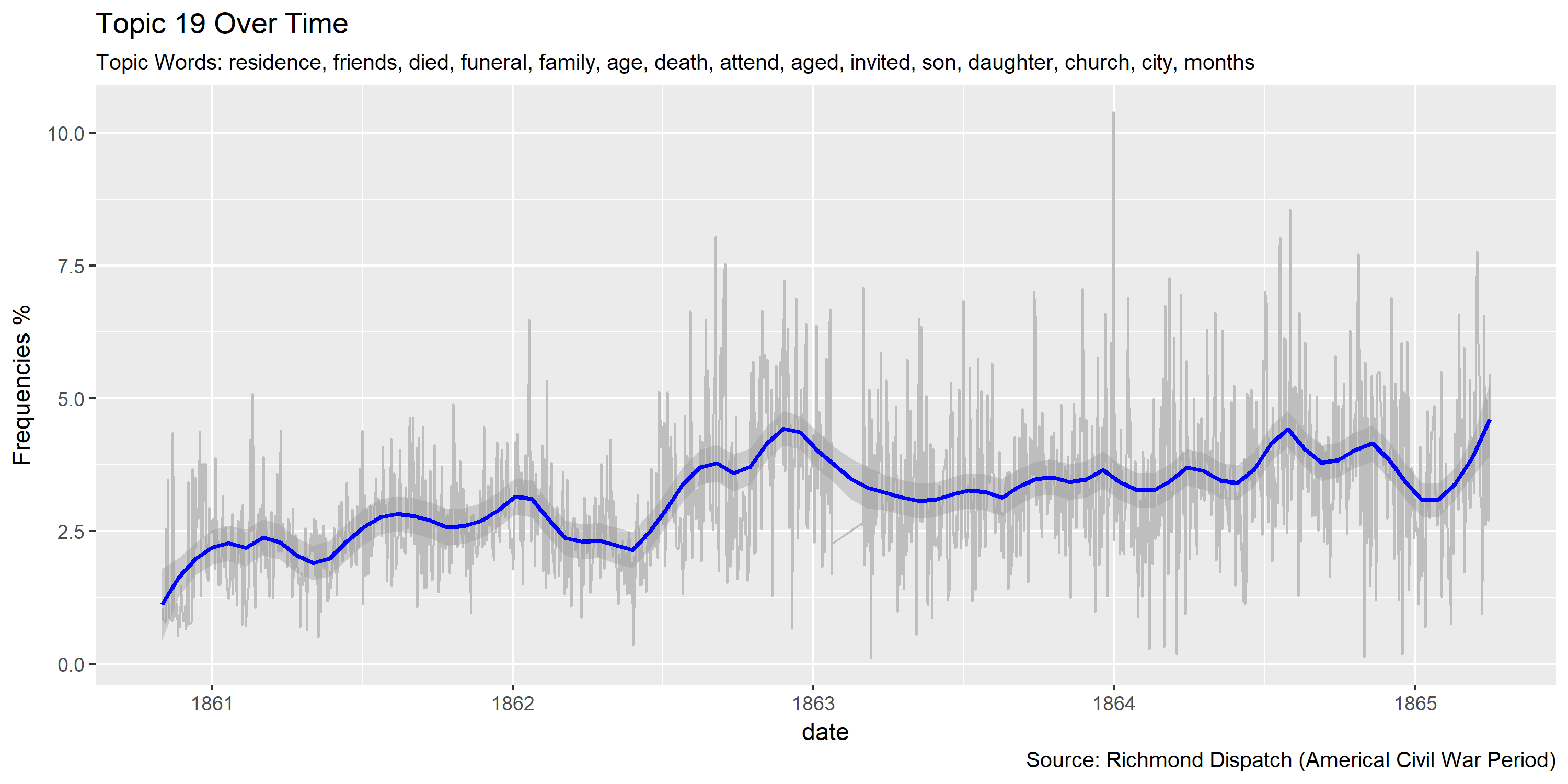
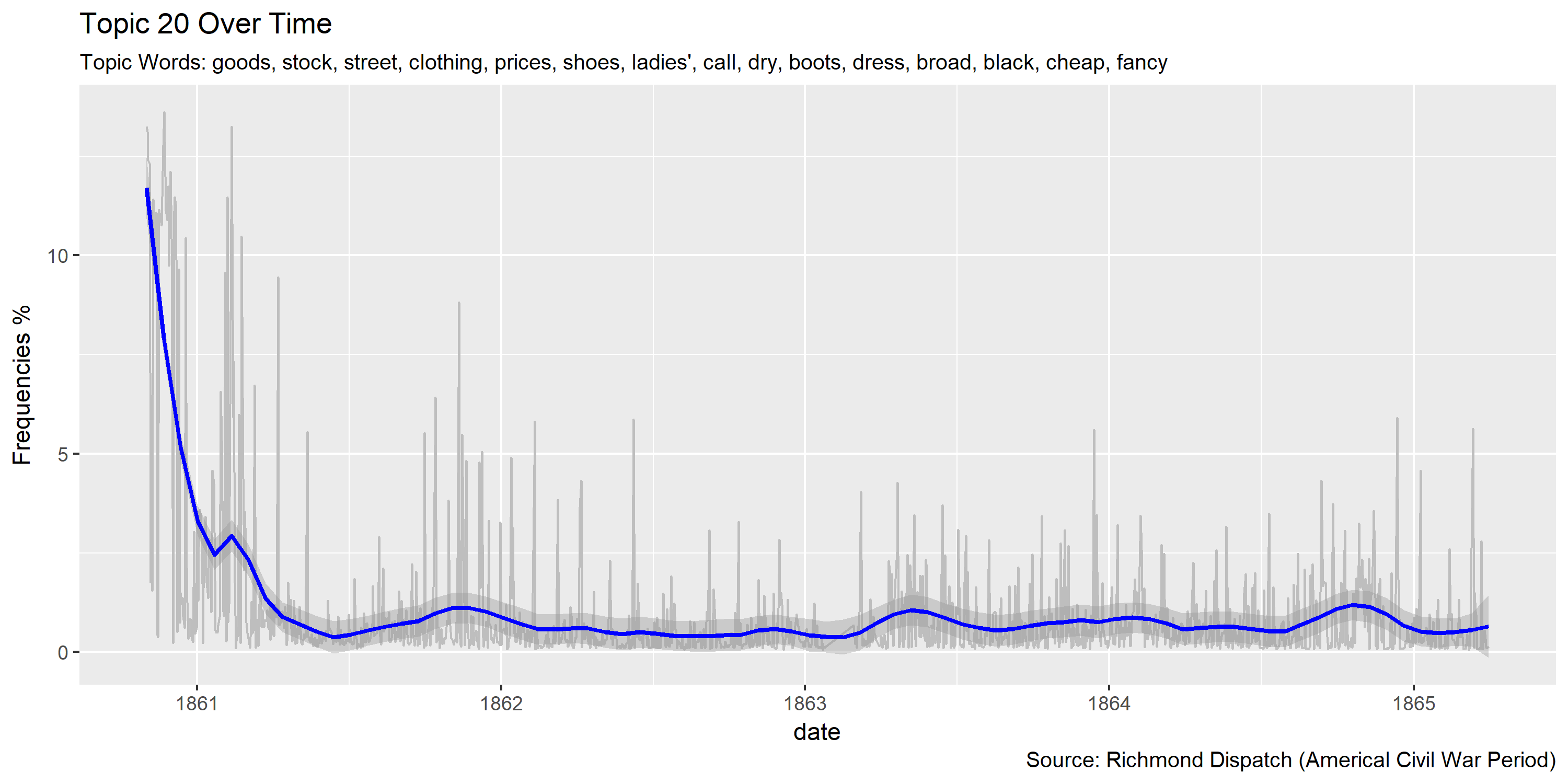
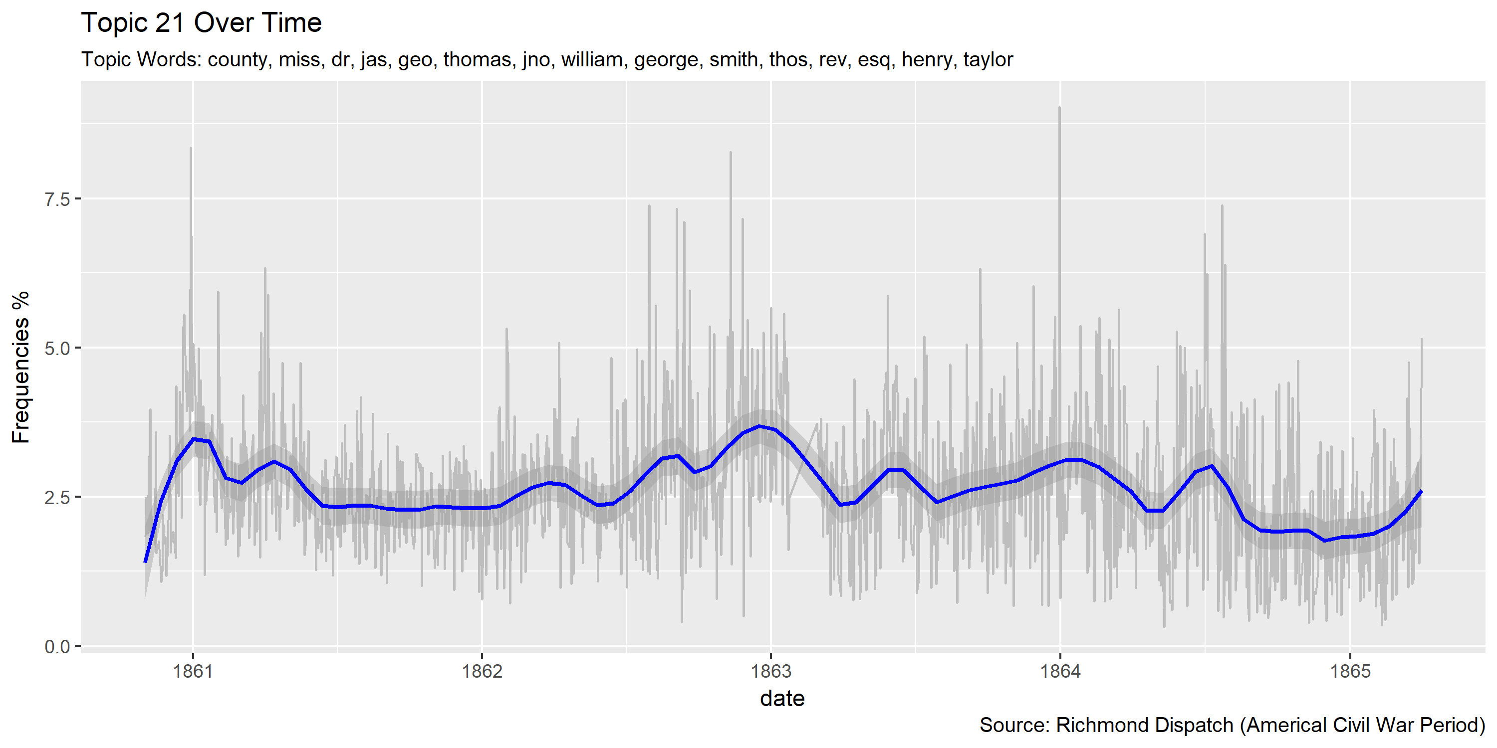
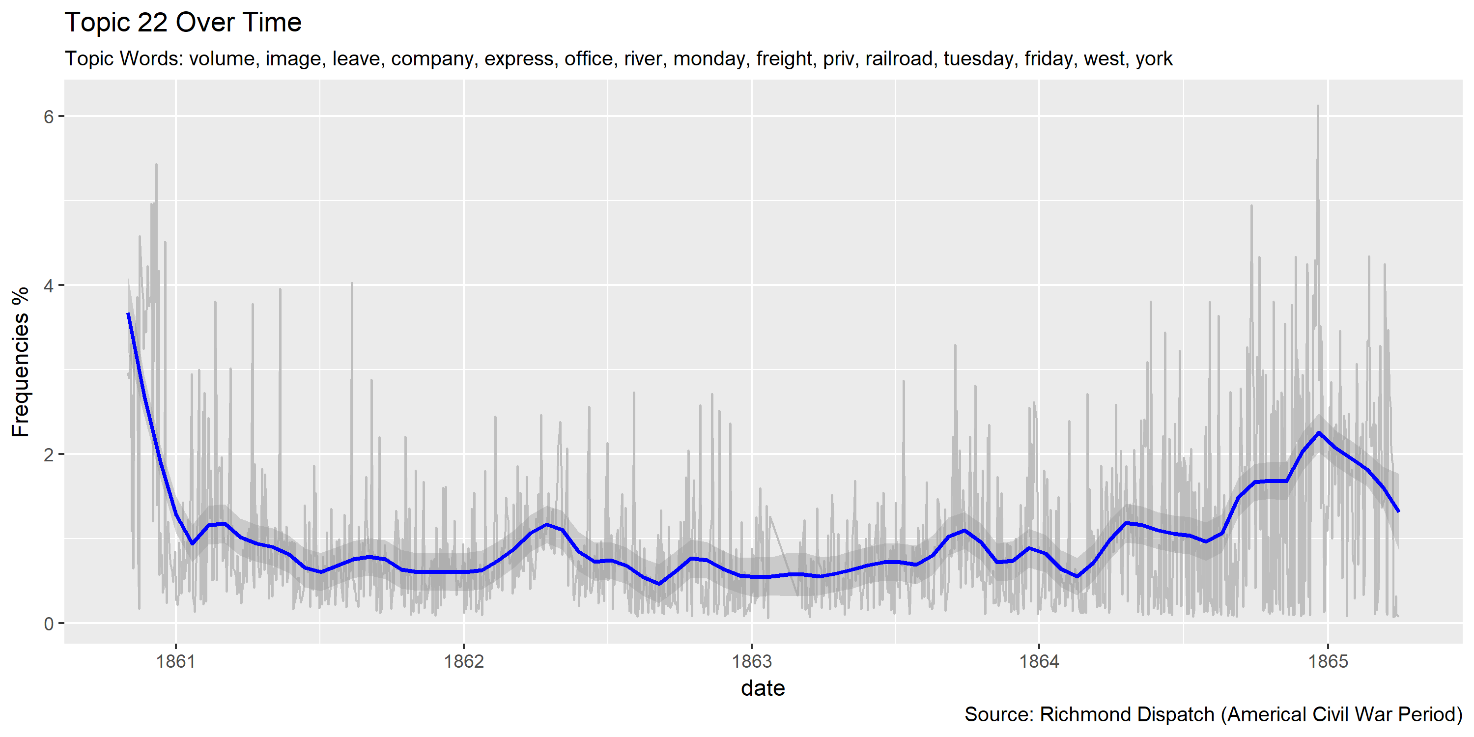
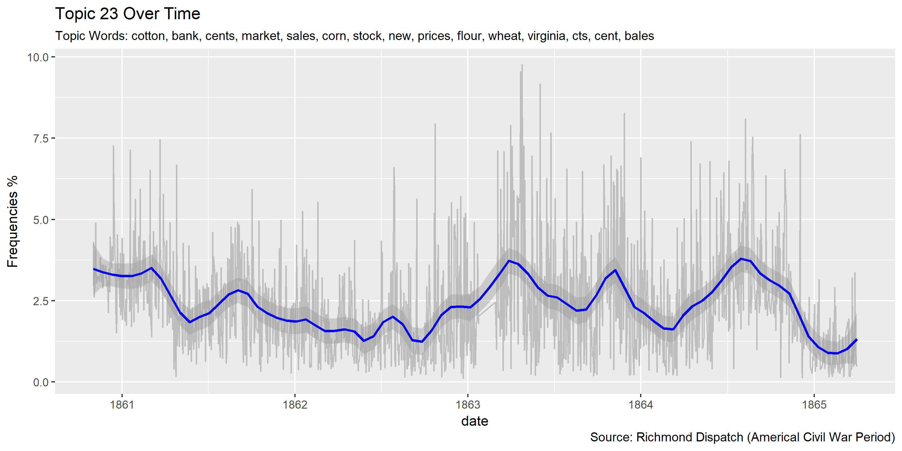
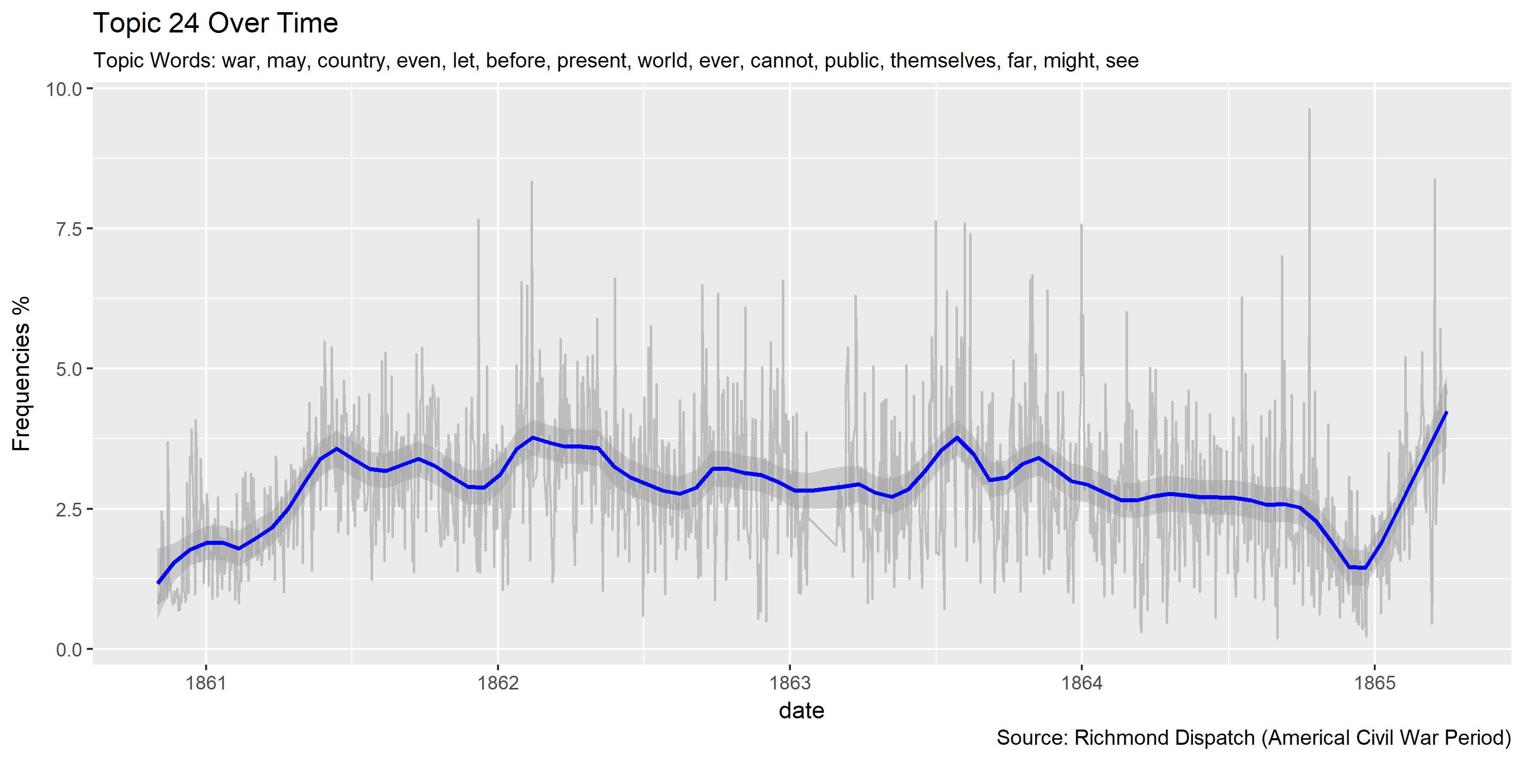
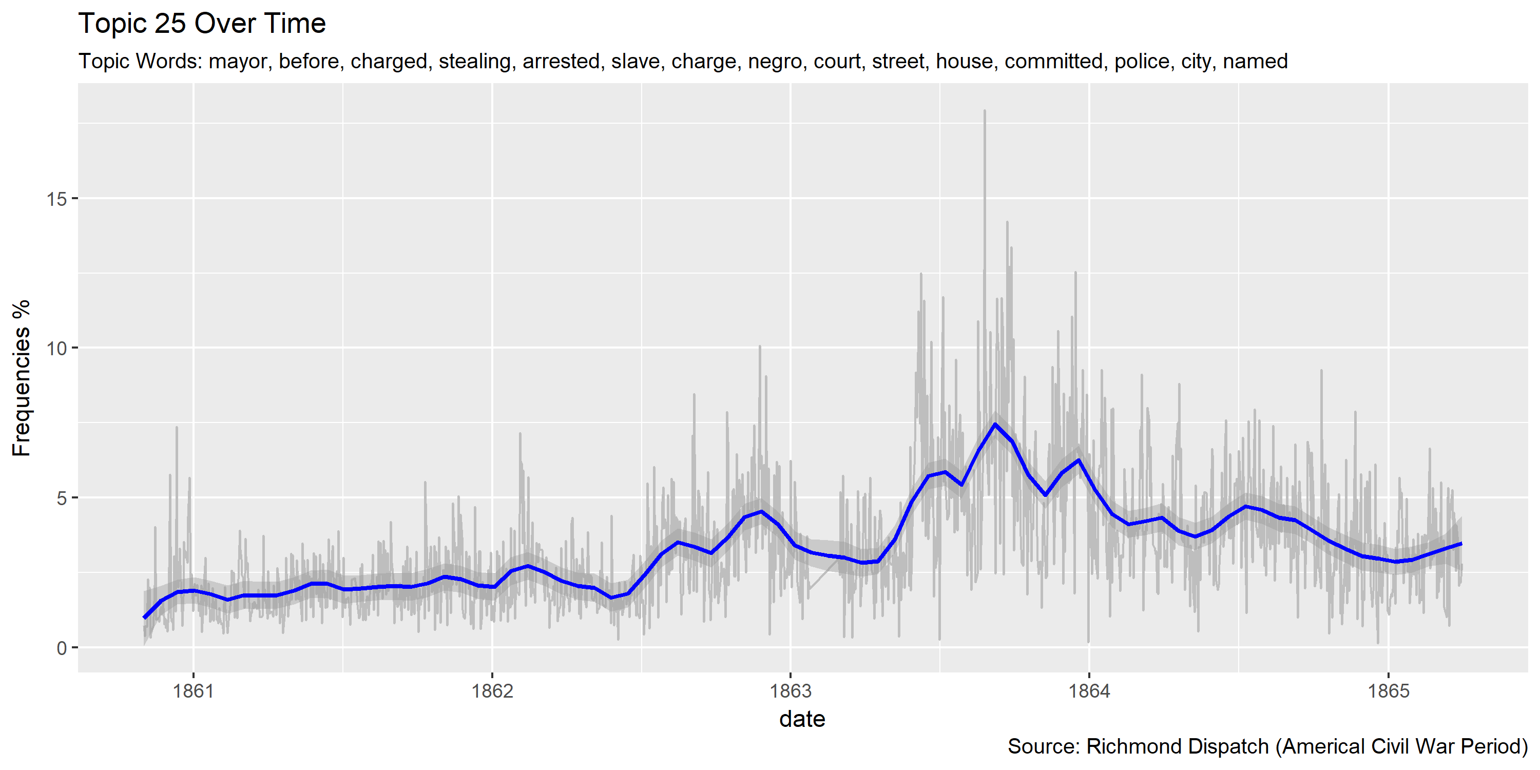
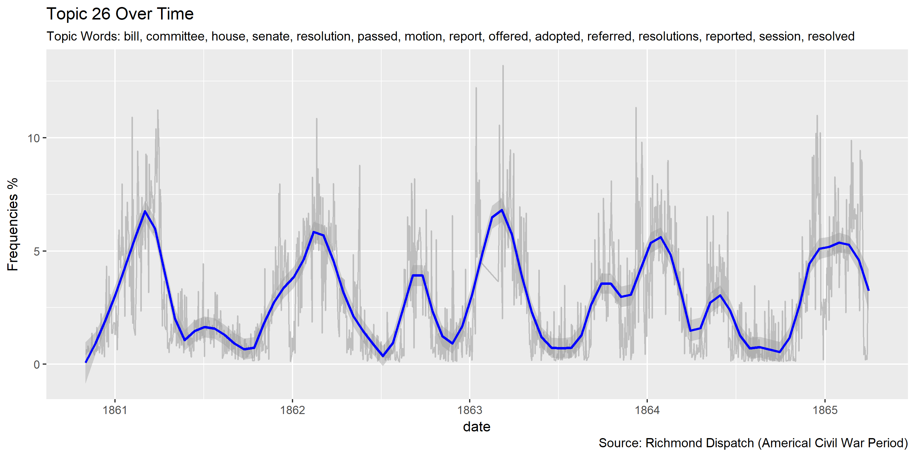
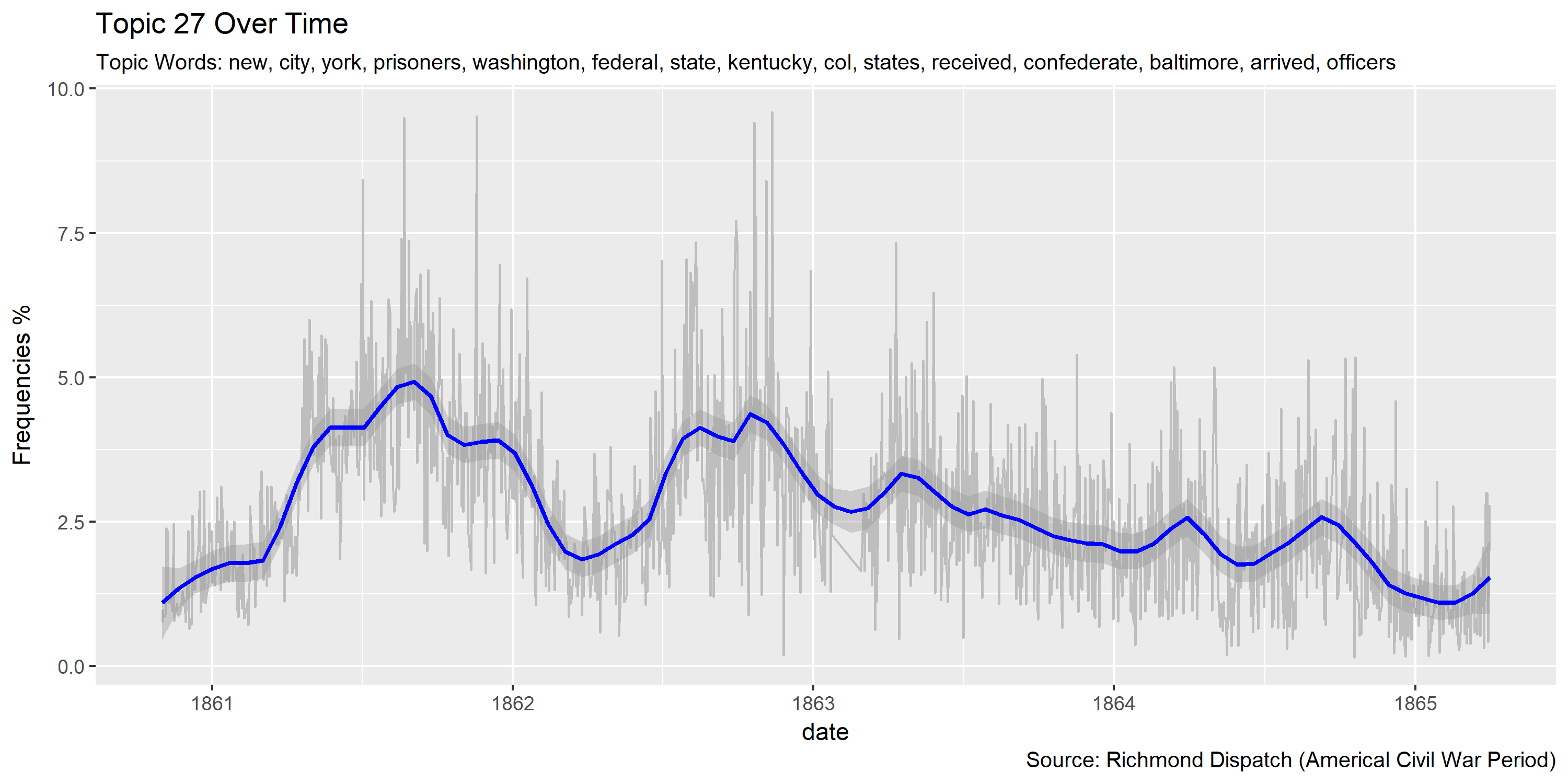
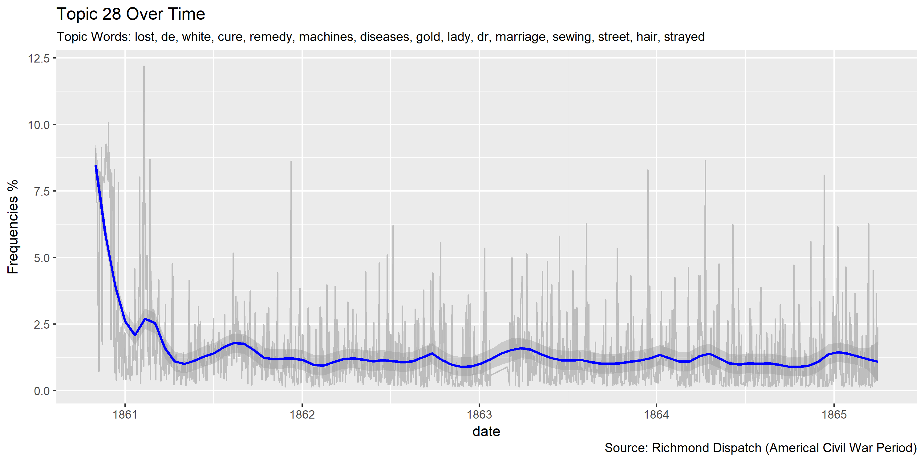
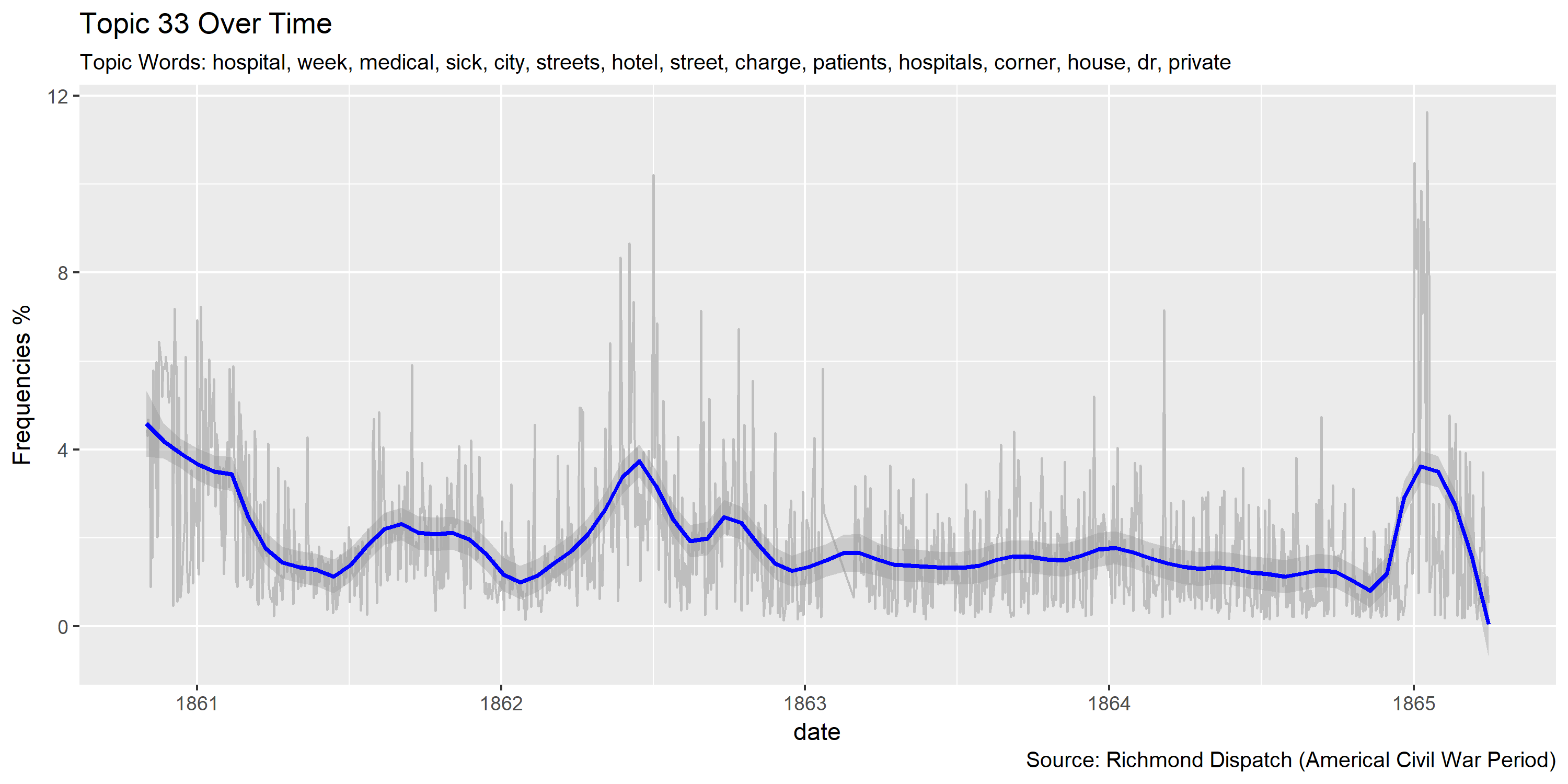
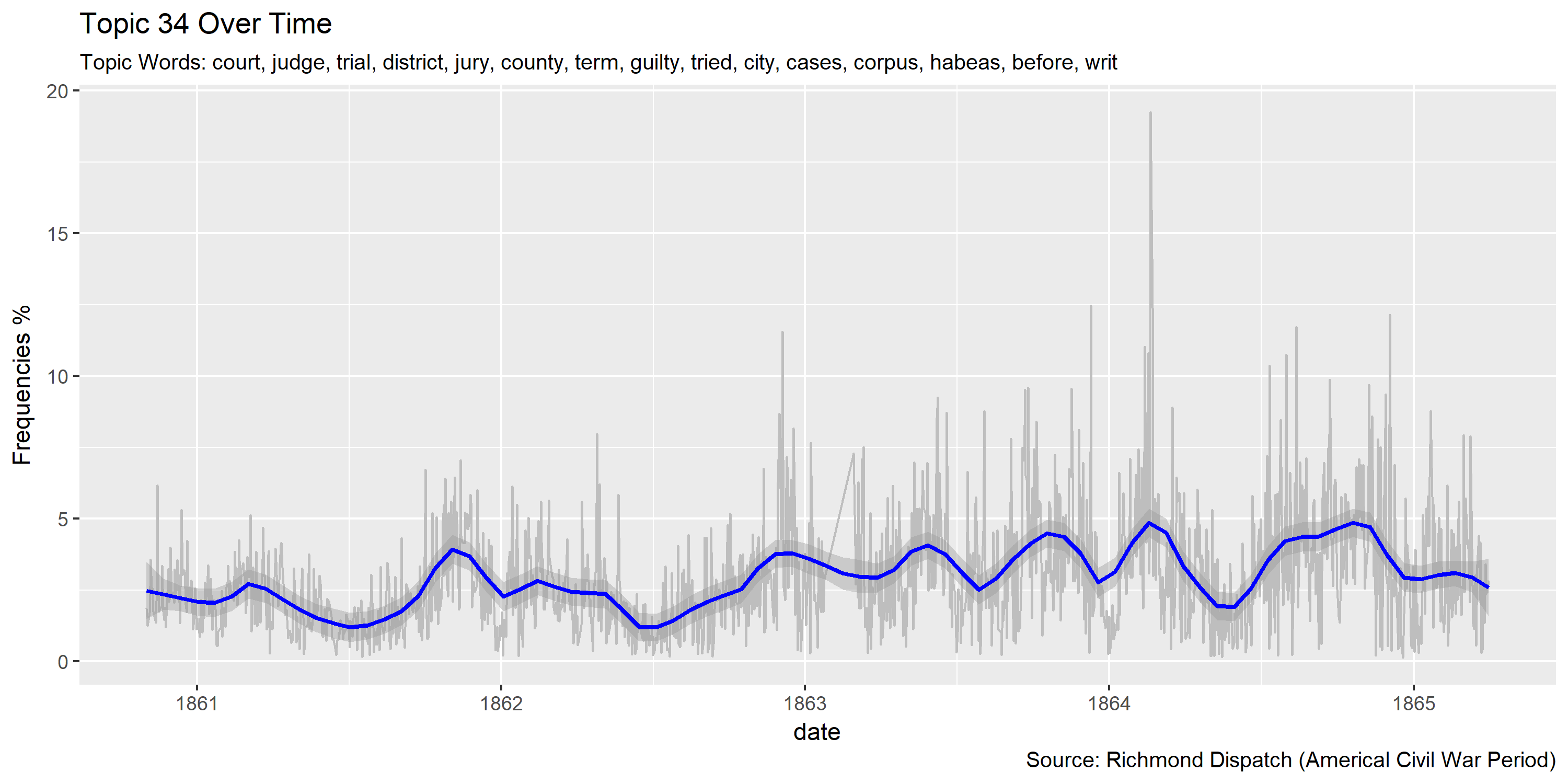
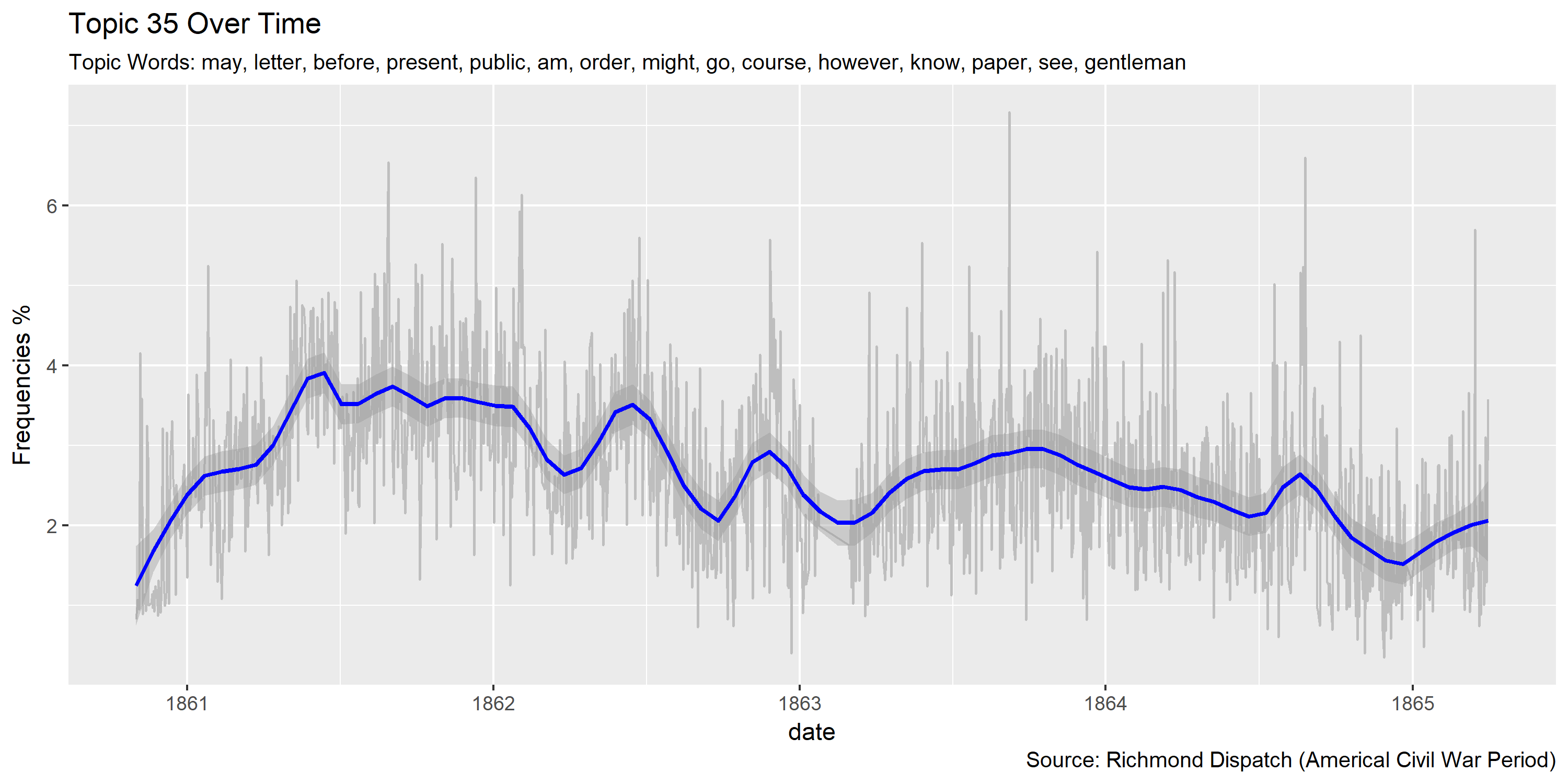
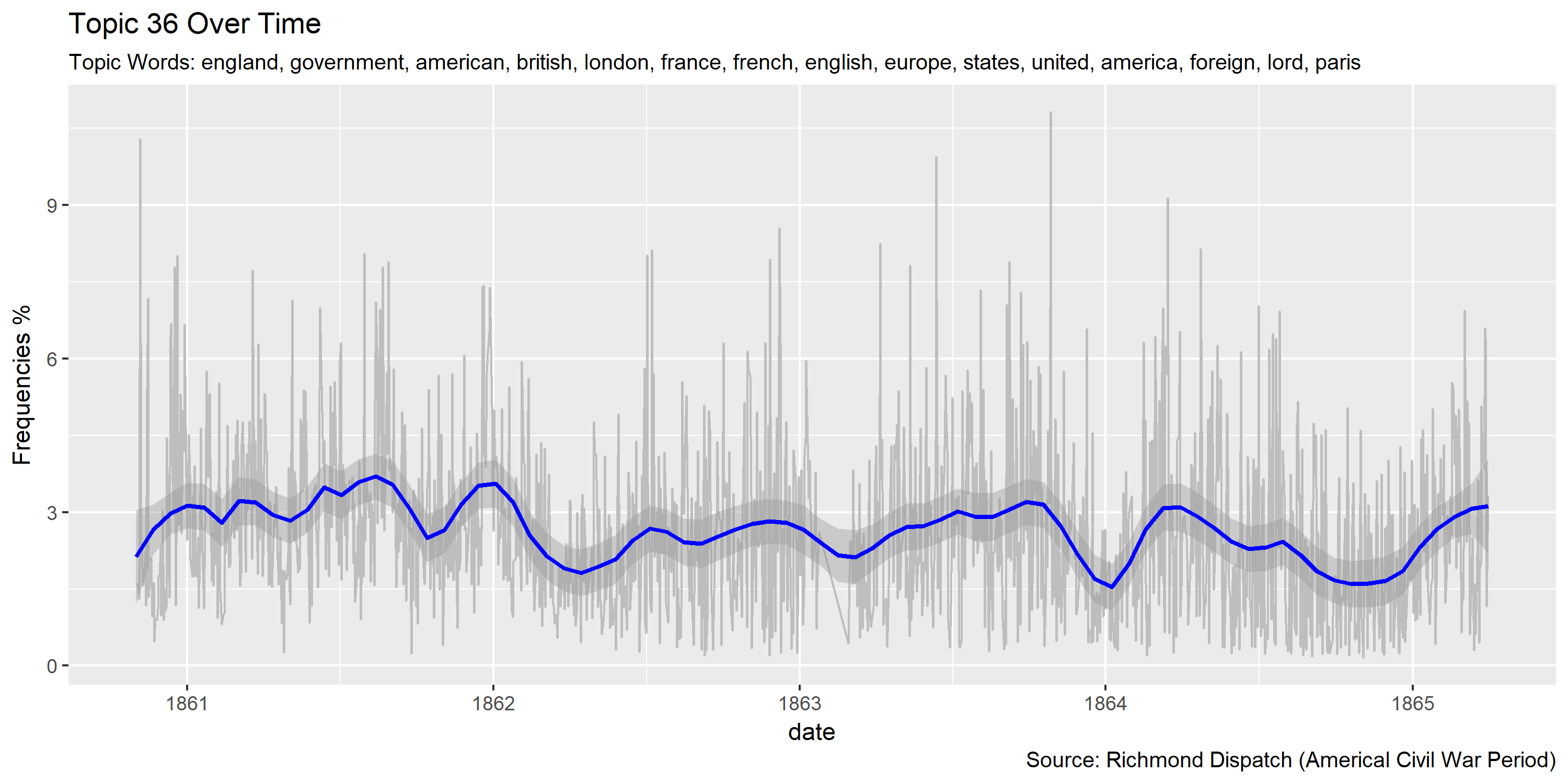
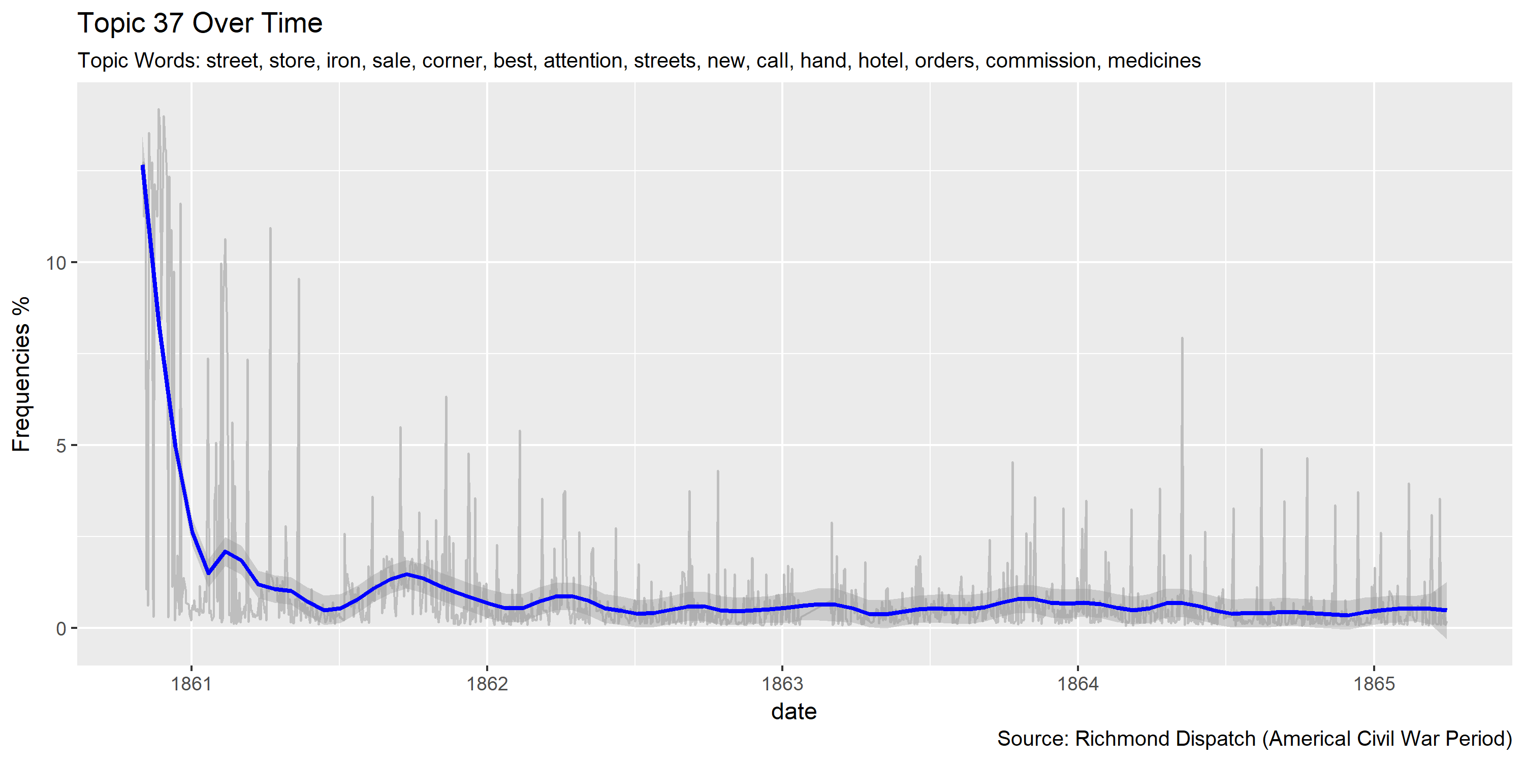
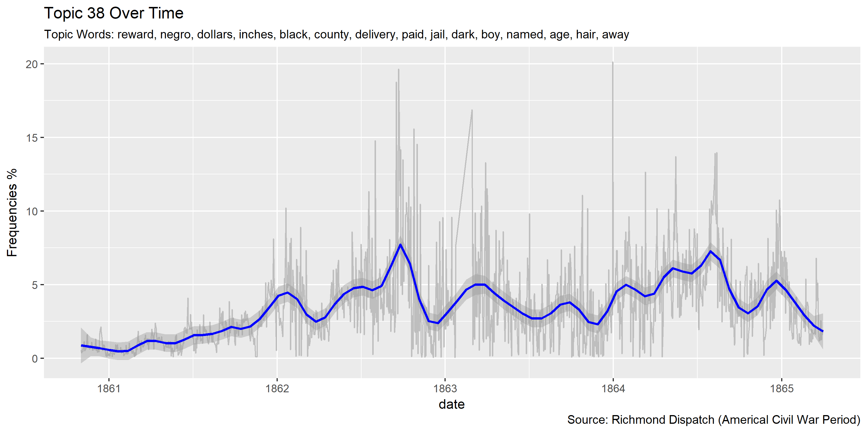
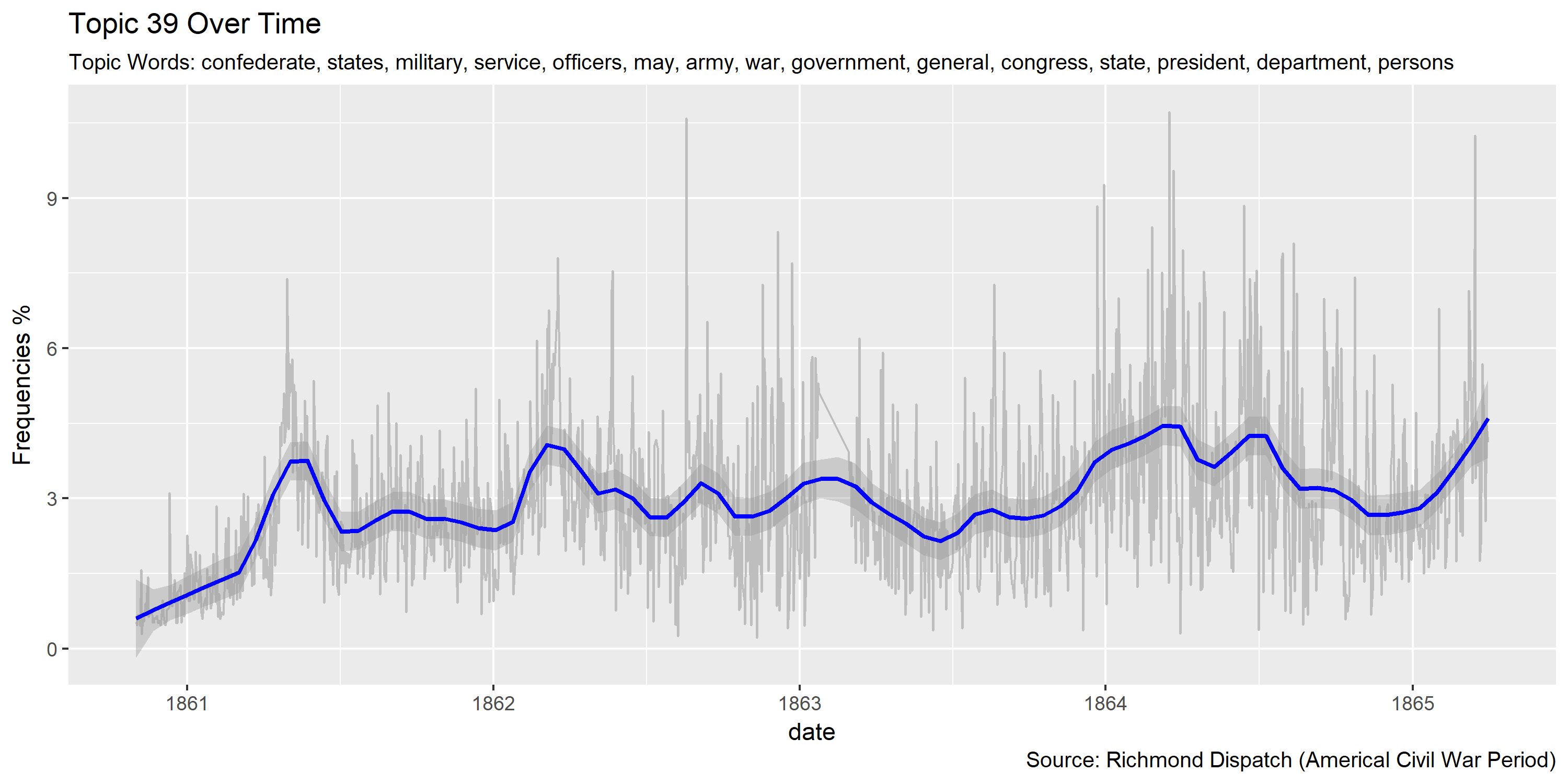
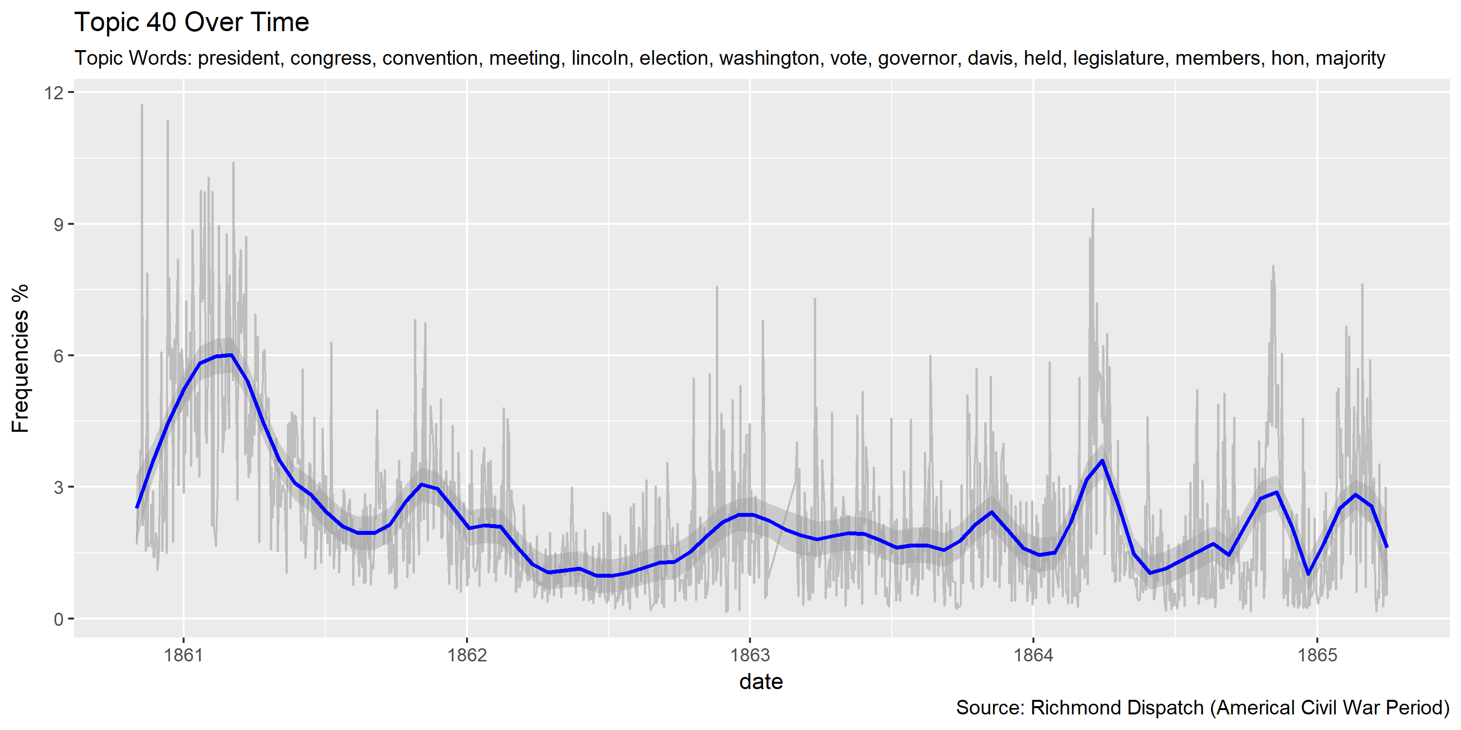
Visualization of topics over time
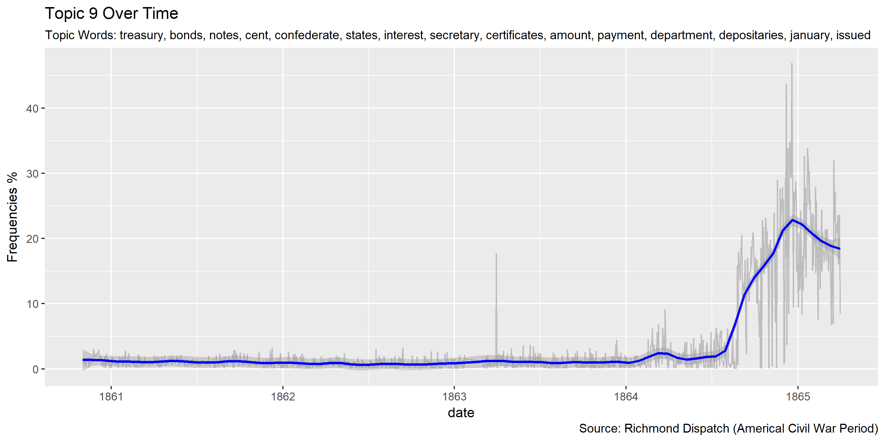
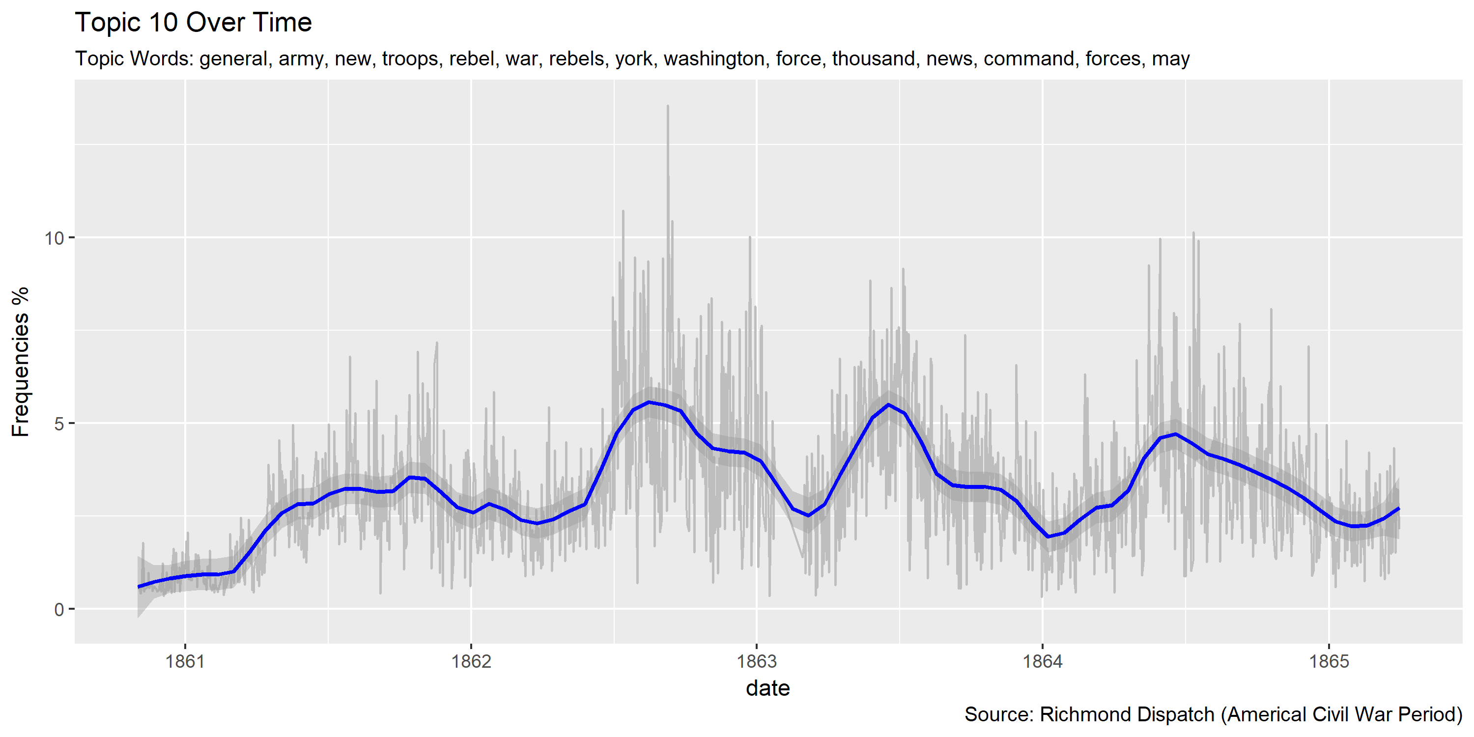
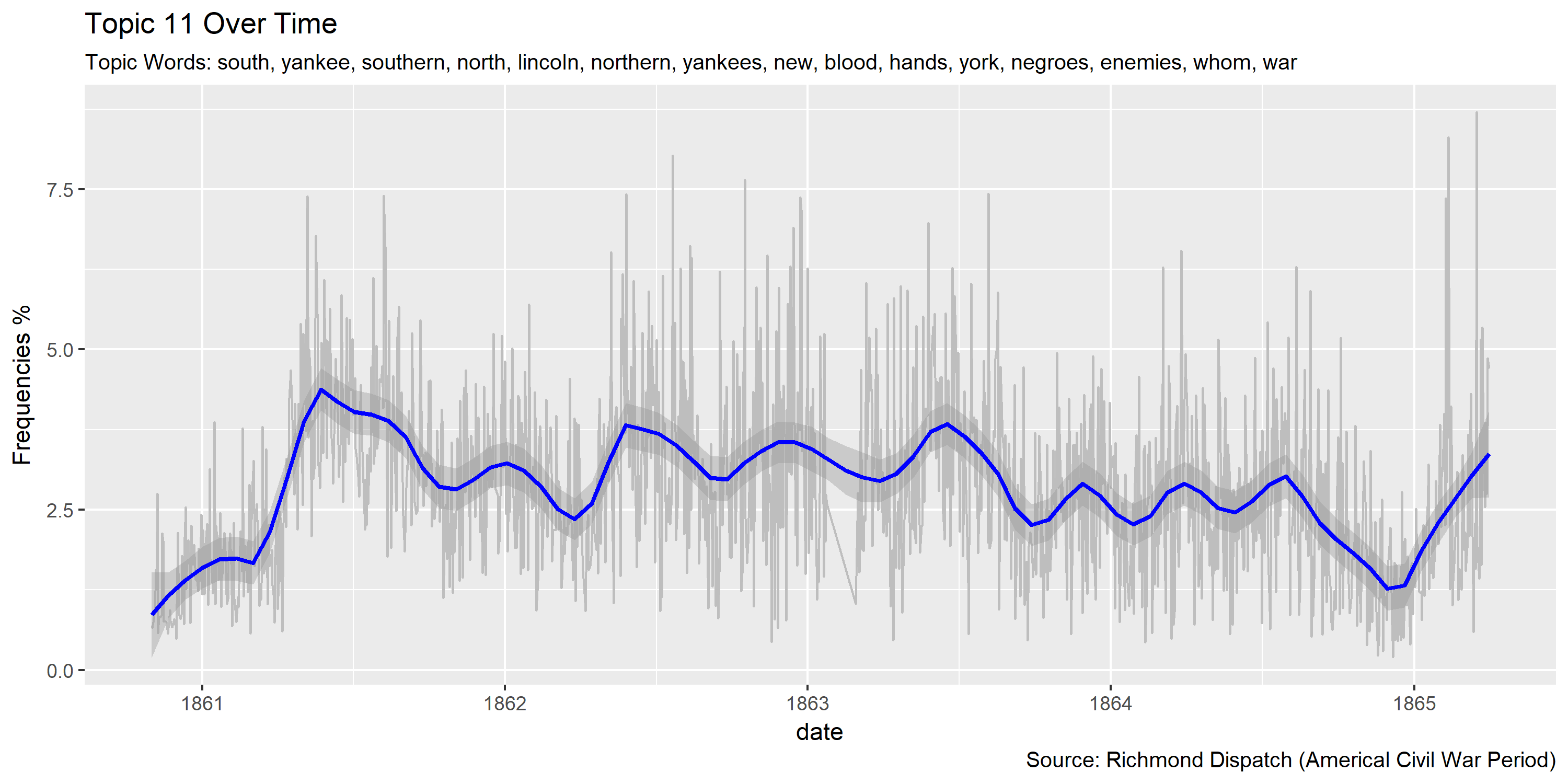
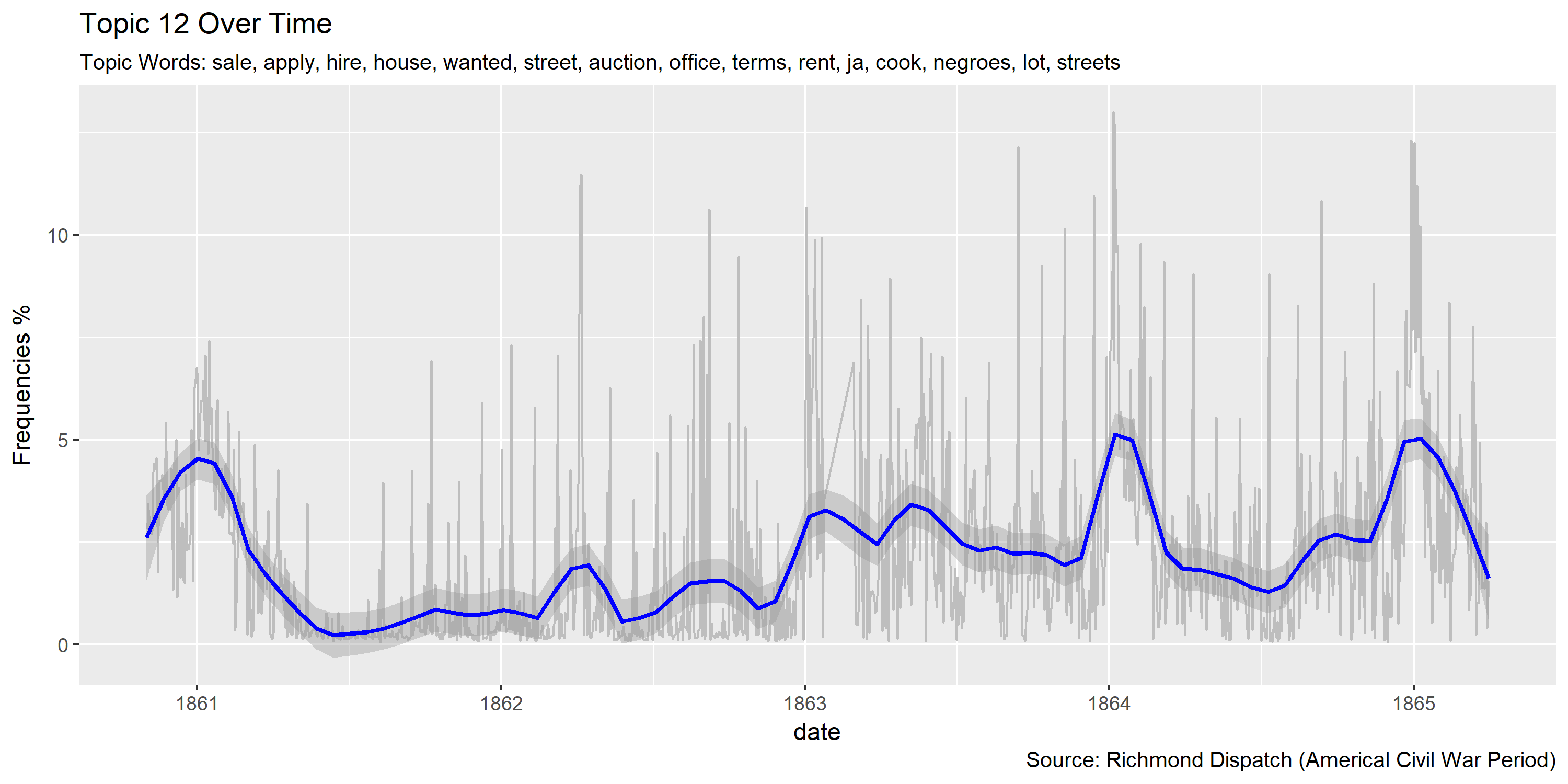
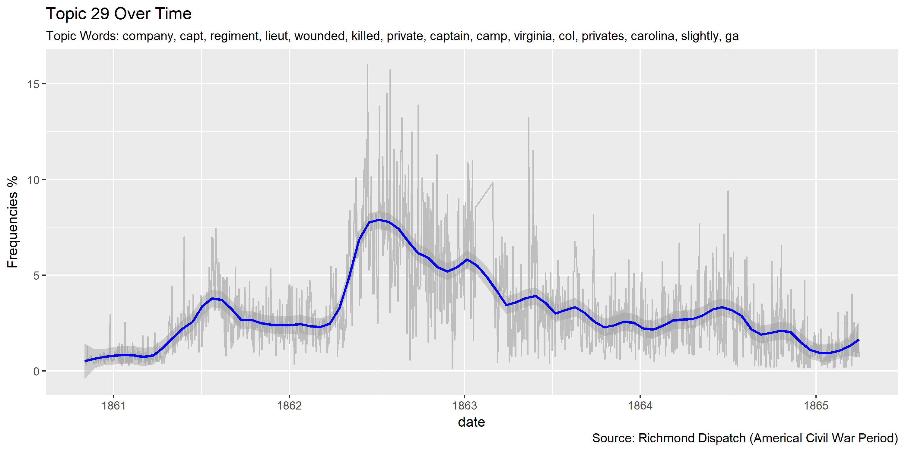
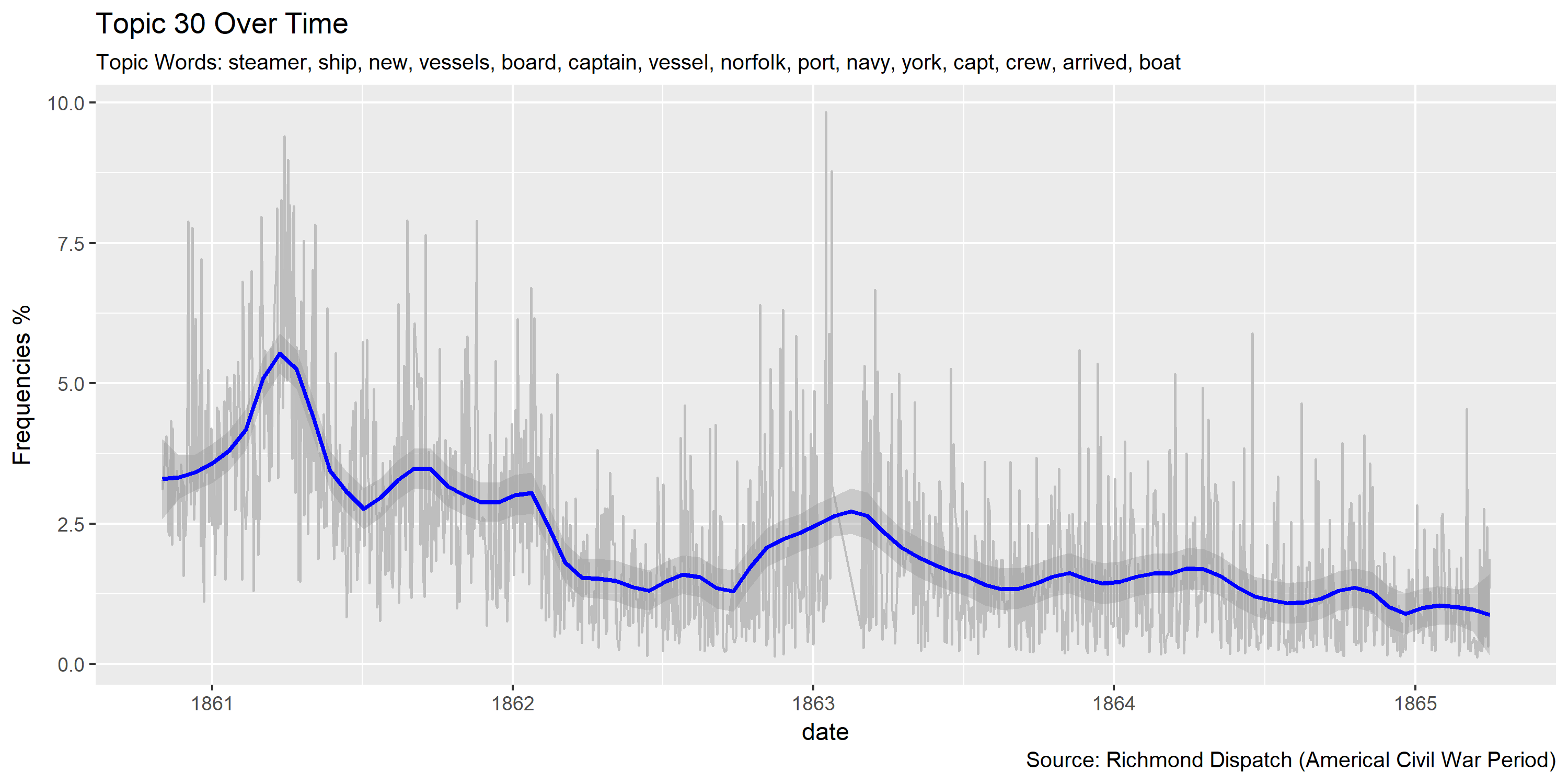
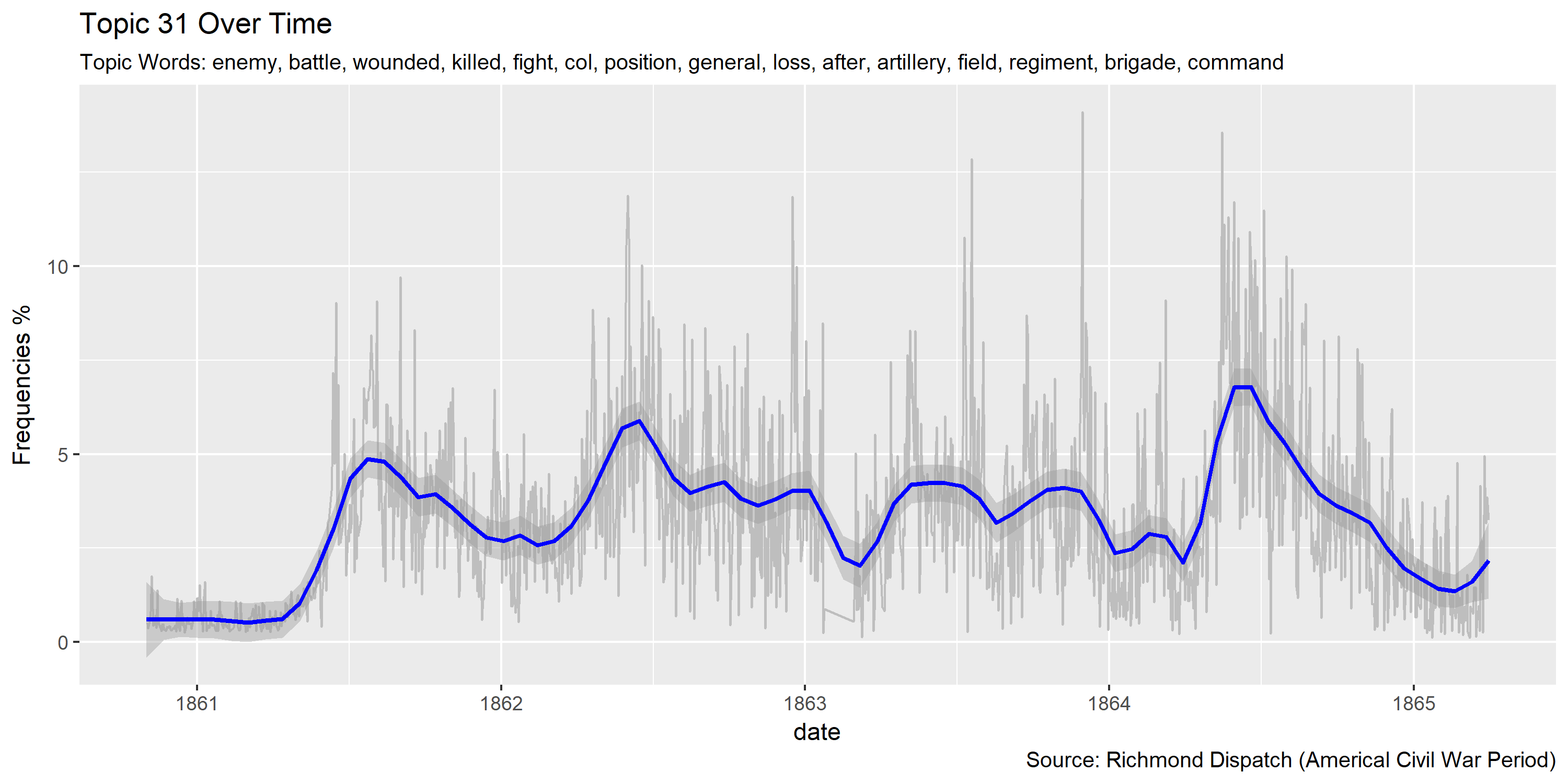
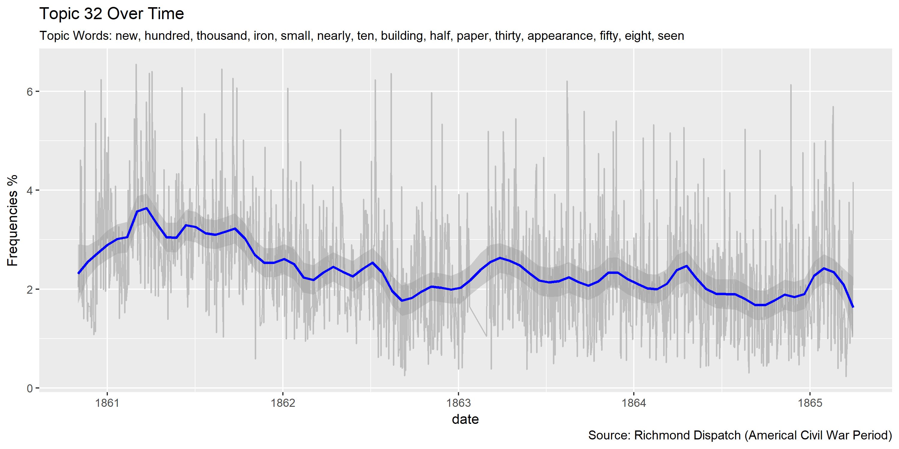
Reference Materials:
- On topic modeling: Blei, David M. 2013. “Topic Modeling and Digital Humanities.” Journal of Digital Humanities. April 8, 2013. http://journalofdigitalhumanities.org/2-1/topic-modeling-and-digital-humanities-by-david-m-blei/.
- More on topic modeling: Brett, Megan R. 2013. “Topic Modeling: A Basic Introduction.” Journal of Digital Humanities. April 8, 2013. http://journalofdigitalhumanities.org/2-1/topic-modeling-a-basic-introduction-by-megan-r-brett/.
- Examples of topic modeling employed by historians:
- Rob Nelson, Mining the Dispatch (http://dsl.richmond.edu/dispatch/)
- Cameron Blevins, “Topic Modeling Martha Ballard’s Diary” Historying, 2010. (http://www.cameronblevins.org/posts/topic-modeling-martha-ballards-diary/)
- David J Newman and Sharon Block, “Probabilistic topic decomposition of an eighteenth century American newspaper,” Journal of the American Society for Information Science and Technology vol. 57, no. 6 (April 1, 2006): 753-767.
- Alternative way to run topic modeling: Graham, Shawn, Scott Weingart, and Ian Milligan. 2012. “Getting Started with Topic Modeling and MALLET.” Programming Historian, September. https://programminghistorian.org/lessons/topic-modeling-and-mallet.
Homework:
- Topic modeling the “Dispatch”: using the provided R-script, run topic modeling on the “Dispatch”.
- Change the number of topics to 30 and compare new results with the results for 40 topics. Record your observations.
- Publish your observations as a blogpost on your website; compare your results with those of Rob Nelson’s Mining the Dispatch (http://dsl.richmond.edu/dispatch/).